Lab 3: Time Series Analysis

The goal of this lab is to provide some basic analysis tools that can be used to process acoustic data time series: filtering, power & energy calculations, receive levels of CW signals, and correlation processing.

Acousonde^TM data from Lab 2A will be used for this lab.

 

Required tools: MatLab, MatLab Signal Processing Toolbox

Rev. 2/8/11

Signal Detection

Cross-Correlation.

When a signal is exactly known, the optimal signal processing detector is based on cross-correlation, searching for the known signal in the received data (signal + noise).

 

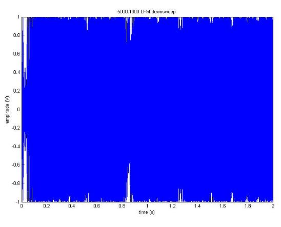
a) Read in 10s of Acousonde^TM data from Lab2A (starting at 06Aug10 16:29:21), and apply a Butterworth, high-pass filter at cut-off frequency of 1kHz.

[B,A]=butter(4,1e3/(fs/2),'high'); % 4th order HP Butter worth filter coefficients

 

b) Calculate received (band level) energy of the filtered LFM time-series.

c) Apply the TL value calculated in Question 3 above to estimate the Source Level (SL) of the LFM signal.

Signal Bandwidth = 1000 Hz to Nyquist rate of data (fs/2) in this case

BL = SPL + 10logBW

4)

References:

Clay & Medwin, Acoustical Oceanography, Principles and Applications, John Wiley & Sons, Inc., New York, 1977.

Kinsler & Frey, Fundamentals of Acoustics, 4th Ed., John Wiley & Sons, Inc., New York, 2000.

Urick, Principles of Underwater Sound, 3rd Ed., Peninsula Publishing, California, 1983.

Still needed (for completeness):

 

Calibrate arrival structure energies so actual TL values can be measured, rather than relative receive energies for cruise data projects.

 

LFM correlation gain of 10*log10(BW) evaluated, is theoretical gain being achieved in the received data?

 

Ideally, rather than signal energies, use Energy Flux densities be calculated/validated to match the RMS SL value from 2 different methods.