Lab 4: Modeling

Lab 4: Acoustic Modeling with Bellhop and NSPE

Goal: The purpose of Lab 4 is to familiarize the students with the implementation of two commonly used propagation models that predict the acoustic pressure fields in ocean environments: Bellhop and the Navy Standard Parabolic Equation (NSPE) model. Bellhop is a ray-tracing model developed by M. Porter and H. Buckner. NSPE is a parabolic equation model that uses the Range-dependent Acoustic Model (RAM) developed by M. Collins as its core engine. These models are available to assist in the analysis of the acoustic environment encountered during the class cruise.

Rev. 2/2/11

BELLHOP:

To start, make a work folder on the C:\ drive (ex: work_Smith).

Copy the files from Lab4_Input folder from the Lab 4 website. These files are needed to demonstrate the execution of various components of the model. Once you have copied the files, open Matlab and make this work folder your Current Folder.

You will be turning in all figures generated, so make sure you save them as they are generated. Note: to help prevent accidently overwriting a new figure onto the current figure's axis, you can precede any of Bellhops's plot commands (plotssp, plotray, plotshd, etc) with the figure command (eg, figure; plotray 'rayfile') to write into a new figure window.

Lab 4 requires the use any of the four computers in the Ocean Acoustics Lab located in SP-315.

These have the necessary paths established in order to run the models without problems.

Plotting sound speed profiles and ray tracing

The input (aka, environmental) file MunkB_ray.env should be in your work folder. Open this in the Matlab editor (or use a text editor like WordPad) to examine its contents. Pages 6-7 of the Bellhop Manual describe the contents and format in detail. Use the link on the desktop to open/review this material.

After reviewing the above, in the Matlab command window, type: bellhop 'MunkB_ray'. An output file MunkB_ray.prt is generated that describes the input in clear format. Open this file with the Matlab (or WordPad) editor and review its contents. This output file is useful for troubleshooting as it will stop when it encounters an input that is does not recognize.

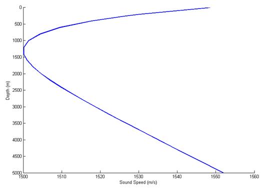
To plot the sound speed profile, type: plotssp 'MunkB_ray' in the Matlab command window. This will generate the sound speed vs depth profile in a Matlab figure (see fig 1).

By now, you've probably noticed the importance of being consistent with the names of related files. You will need to keep this in mind when generating your own files with your own data.

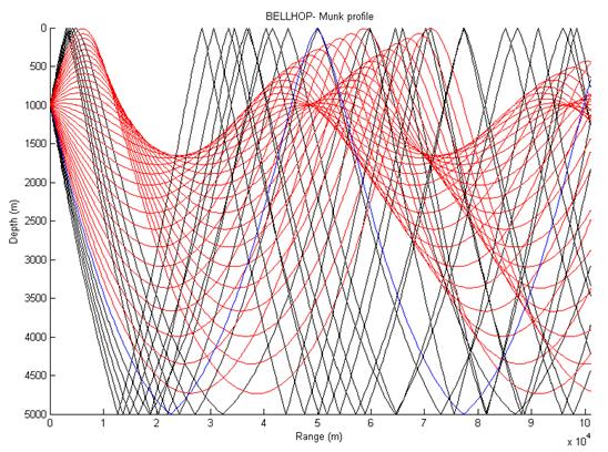
When you ran the bellhop command above, you also generated a file called MunkB_ray.ray. This file contains the ray trace information which you can now plot executing plotray 'MunkB_ray' at the Matlab command window. This will generate a new figure (see fig 2).

Plotting eigenrays

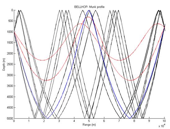
Open the file Munk_eigenray.env with the Matlab (or another text ) editor and review its contents. It should be located in your work folder. Read page 13 of the Bellhop Manual. This explains in more detail why you use the number and type of rays, and single source and receiver at a single range.

After reviewing this, execute the bellhop and plotray functions using this environmental file as the input. You should get the same as fig 3.

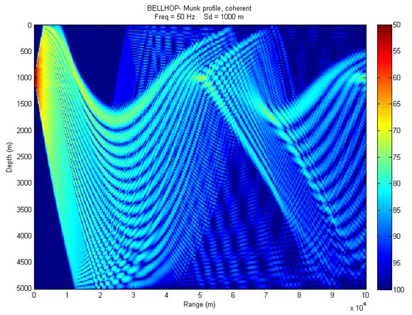
Read the last sentence on page 18 and all of page 19 of the Bellhop Manual. Edit the MunkB_Coh.env file to make the change to Gaussian beams as suggested in the last paragraph of page 19 (ie, change run type from "C" to "CB") and rerun bellhop and plotshd to make the figure shown as fig 5.

Plotting transmission loss (TL)

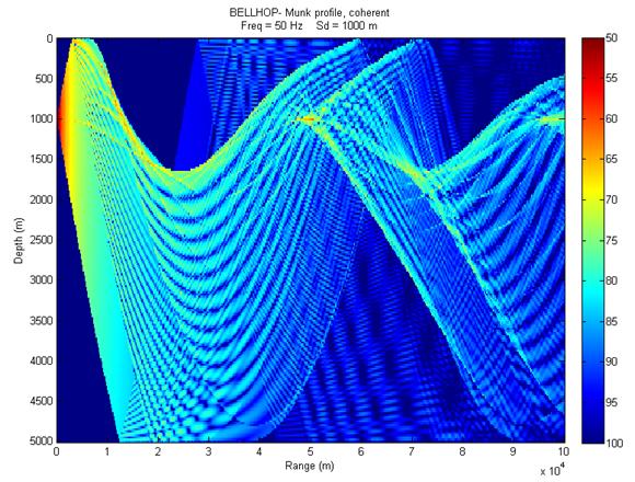
Open the file MunkB_Coh.env (should be in your work folder) and review its contents. Read page 17 and the first paragraph on page 18 of the Bellhop Manual which explains the important settings used to make a coherent TL plot.

After reviewing the material above, execute the bellhop function on this input file. This will generate a file called MunkB_Coh.shd. Now run plotshd 'MunkB_Coh.shd' to generate the figure shown in Fig 4 (note the extension .shd must be included).

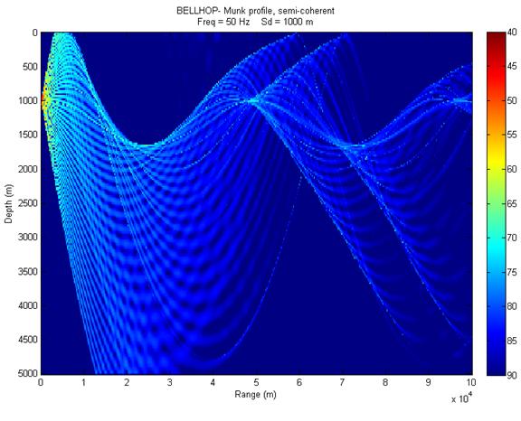
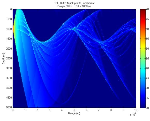
Read page 21 of the Bellhop Manual. Making the necessary changes to the MunkB_Coh.env file, run bellhop and plotshd to make semi-incoherent and incoherent TL plots using only geometric beams (see figs 6 and 7). You should also change the title (line 1 of the .env file) to match the run type. You can also do this "after the fact" using title('new plot title') at the Matlab command prompt on the current figure.

Plotting bathymetry

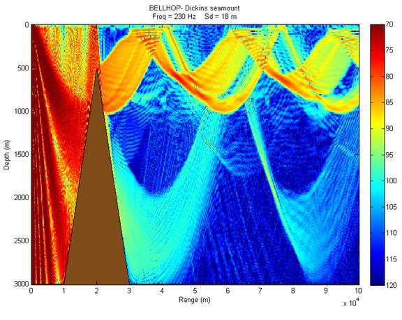
Open both the DickensB.env and DickensB.bty files to review their contents. Read page 27 of the Bellhop Manual and note how the key points are implemented in the opened files.

After reviewing the material above, execute bellhop and use plotshd to display TL. To add bathymetry, use plotbty 'DickinsB' to match figure 8.

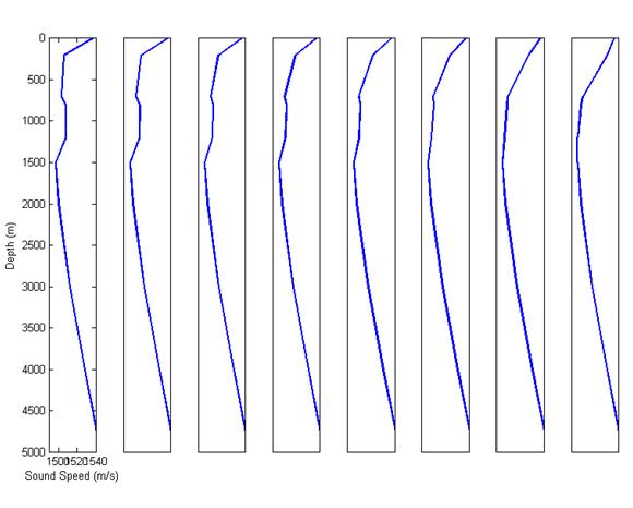
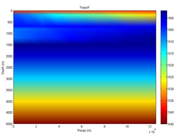
Range-dependent SVPs

Review the material on pp 37-39 of the Bellhop Manual. By now, you should have the gist of how to execute Bellhop.

Run the Gulf_ray_rd example (the required .env, .ssp and .bty files should be in your work folder) using the plotssp2D function to plot the range dependent profiles and profile surface as shown in figs 9 and 10. Note you may have to "stretch" your multi-profile figure to see them correctly (ie, make the figure much wider than tall on your screen).

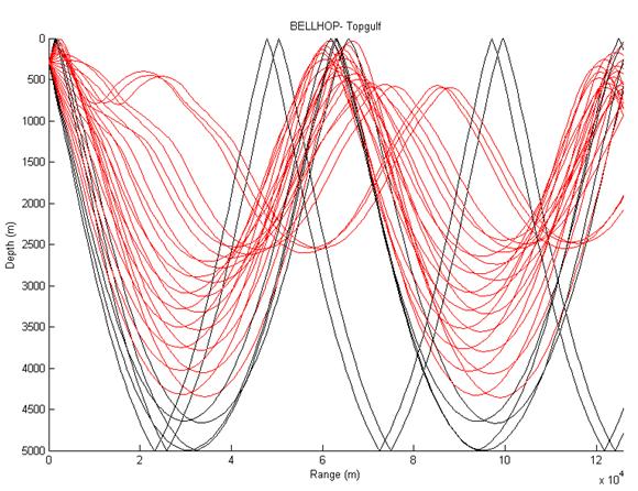
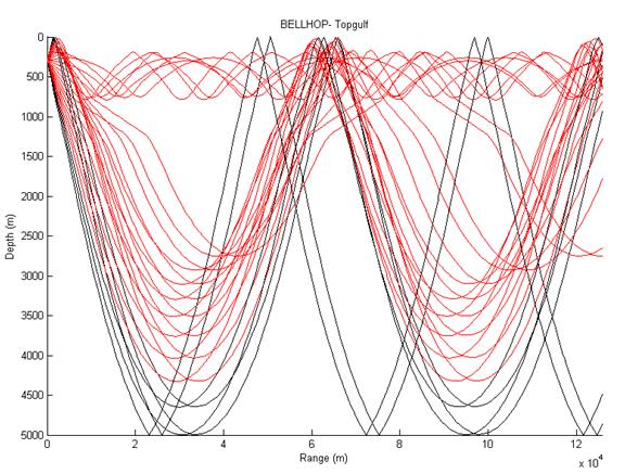
Run bellhop and plotray to generate the range-dependent display (see fig 11).

Change the 'Q' to 'C' on line 4 of the .env and re-run the range-independent case (this causes Bellhop to use only the profile in the .env file). Plot the results to get fig 12.

At this stage, you've become familiar with many of the features that can be executed in Bellhop. However, there are many more options that could be run. Open the General Description Manual and go to section 5 (Input and output files) where it lists other options that could be applied. There's not enough time to execute all of these, but this is a good reference in case there are features that you may want to use in your analysis work.

Absorption:

On page 6, Option1(4) is an important feature to exercise. This is the 4^th character in line 4, but it was not used in any of the previous examples. This parameter accounts for volume absorption in the water column - it should be a 'T'. I highly recommend you use it...without it, your TL prediction will likely be much less than measured.

Arrival times and amplitudes: these can be computed in Bellhop by changing the run type to 'A' (see Option3(1) on pg 7 of the General Description Manual). This manual guides you through an example (pp 15-16), but there seems to be a couple of errors in the instructions, so we'll do something similar - but different.

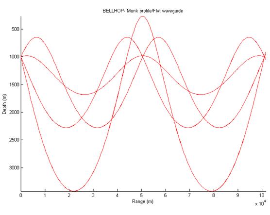
Open the input file called MunK_flatwav.env which has been set up to find eigenrays between a source and receiver, both at 1000m depth and 101 km apart. Run bellhop and plotray to see the eigenray paths. This should look like fig 13, but compare this to fig 3 on page 14 in the General Description Manual. Your plots will have more precise paths because you've used 5001 rays vice their 101 rays.

Now change the Run Type from 'E' to 'A' and re-run bellhop to generate an output file called Munk_flatwav.arr which contains the arrival structure data.

Next run [Arr,Pos]=read_arrivals_asc('Munk_flatwav.arr', 4) which will write two Matlab structure variables (Arr and Pos) in the Matlab workspace. Arr contains all the arrival information and Pos contains the source and receiver position information (ie, depth and range). In this case, there were 4 eigenrays from the plot in 3.h(iii) above, so this number of arrivals was used as an input. If you don't know the number of eigenrays, you can leave this input off and it will default to 200 which adds a lot of zeros to the Arr matrix...but otherwise no harm done.

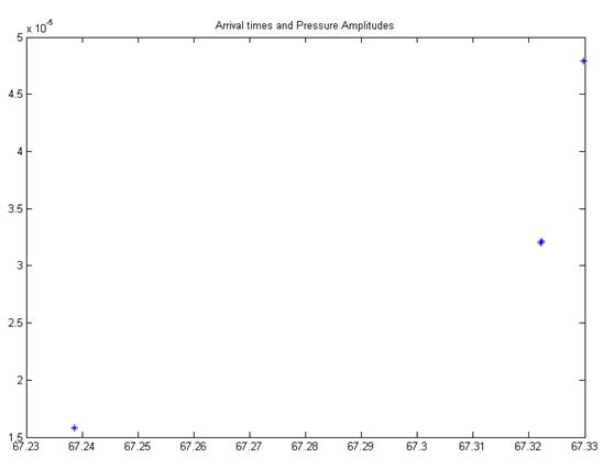
Double-click on Arr in your workspace to see the following variables:

Arr.A - complex pressure amplitude of each ray at the receiver

Arr.delay - travel time in seconds from source to receiver

Arr.SrcAngle - angle at which the ray left the source (pos is down, neg is up)

Arr.RcvrAngle - angle at which the ray is passing through the receiver

Arr.NumTopBnc - number of sfc bounces

Arr.NumBotBnc - number of bottom bounces

Arr.Narr - number of arrivals

Plot the travel time vs magnitude of the complex pressure of the 4 eigenrays and turn in (see fig14) using the following code:

figure; plot(Arr.delay,abs(Arr.A),'*');

title('Arrival Times and Pressure Amplitudes');

Use Lab 1 sound speed profiles, bathymetry and one EMATT leg to show eigenrays from the EMATT (at its farthest point) to the Acousonde. Use 1 kHz. Turn in figure.

Save and turn-in a copy of all figures (Figures 1-14)

Congratulations! You're done with Bellhop (for now)

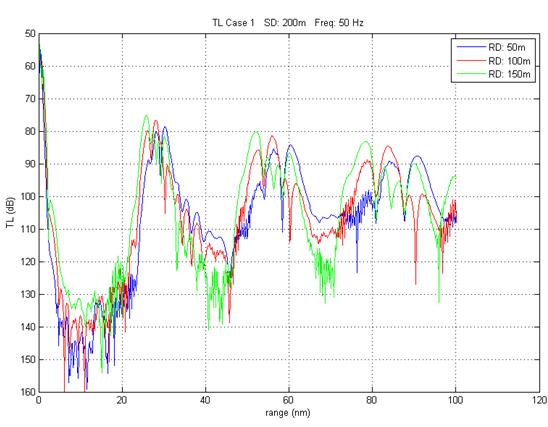
NSPE

To start, open a command prompt window (a link is on the desktop). Change directory to C:\nspe_OC4270. (use cd .. twice to back up to C:\, then cd nspe_OC4270).

NSPE requires an input file called nspe.in to be present where the executable file is. Open the folder C:\nspe_OC4270 (a link called NSPEv5.5 input-output is on the desktop and will take you there). You may see an input file in this folder leftover from the last person that used this computer. If it's not there, that's not a problem because you're going to replace it with ones you make anyway. Leave this window open as you'll be copying your own nspe.in file into here to execute the program.

Open a 3^rd window. This one to your work folder that you were using with Bellhop that contained the input files (eg, C:\work_Smith folder). In this folder, you should have three files with .in extensions (case1.in, case2.in and case3.in).

Open case1.in using a text editor (WordPad or Matlab will work). Review the contents. In this case, the input file describes a fairly simple range-independent (1 SVP) environment over a deep, flat bathymetry and a fully absorbing bottom. The source is omni-directional broadcasting a signal at 50 Hz. The output is three unaveraged TL vs range curves for a fixed source at depth 200m and 3 moving receivers at depths 50m, 100m and 150m (the use of "tl" in the output sections indicates that). Use STD Appendix A (a link to the NSPE documents in on the desktop) starting on page 4 (PE RAM Inputs) to follow the organization of the input file line-by-line.

Copy case1.in into the C:\nspe_OC4270 folder and rename it nspe.in (you may have to delete the file nspe.in that already exists in that folder). In the command prompt window, type nspe_55.exe which will execute the model using this input file. You should see the progress of the model in 10% range increments shown in the command prompt window.

When the model completes, an output file called nspe01.asc is generated. This file is a text file. Review its contents with a text editor (eg, WordPad or Matlab) and you will see 4 columns. The first is range (in nautical miles) and columns 2-4 are unaveraged TL (in dB) for each of the three receivers. Plot range vs TL on a single plot (fig 15). TL is typically plotted with increasing TL in the downward direction. The following code will help make the plot:

load('nspe01.asc')

figure; plot(nspe01(:,1),nspe01(:,2),'b'); grid on;

set(gca,'ydir','r');

hold on; plot(nspe01(:,1),nspe01(:,3),'r');

plot(npse01(:,1),nspe01(:,4),'g'); hold off;

ylim([50 160]); xlabel('range (nm)'); ylabel('TL (dB)');

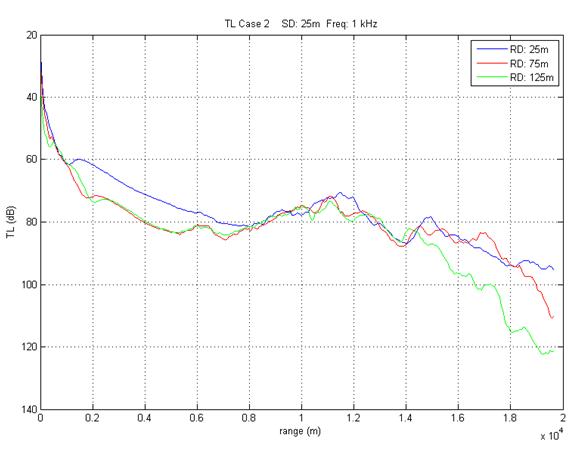
Repeat steps d-f for case2.in making a similar plot (fig 16), but note the following changes:

the frequency is 1 kHz, source depth = 25m, receiver depths = 25m, 75m, 125m

the bottom is not fully absorbing, but uses bottom loss in LFBL format

the output is metric, therefore the range is in meters, not nautical miles

the output type is range-averaged TL (indicated by "rtl") so the output is written to a file called nspe02.asc.

Plot range-averaged TL for all 3 receivers on the same graph.

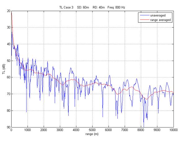
Repeat steps d-f for case3.in but note the following changes in the input file:

freq = 800 Hz, source depth = 60m, receiver depth = 40m (only 1 this time)

bottom loss is based on a geoacoustic model using the following parameters: bottom compressible sound speed, density and attenuation (all vs. depth)

surface scattering losses accounted for by range-dependent wind speed

both coherent (tl) and range dependent (rtl) TL are generated. PLOT BOTH on same plot (fig 17)

a full field TL output has been requested (plotting instructions below)

To make a full field plot of TL:

return to the command prompt window and type: nspe_fld which will run a program that pauses and requests 2 additional inputs: the depth (in meters) of the plot you wish to make and how to display the bathymetry (1, 2 or 3).

Type 100,2 <enter> to complete the program. This makes a binary file called fld3c.out that contains the full field TL information.

Open Matlab and make C:\nspe_OC4270 your current directory. Run plot_TLFF.m which reads the full field TL file and makes the plot (fig 18).

Turn in all TL plots (Fig 15-18).

Again, not all possible options in NSPE were exercised, nor is there time to exercise these. However, STD Appendix A is an excellent reference should you need other options to exercise in your analysis.

Congratulations! You're done with NSPE (for now)

A PDF copy of these instructions can be found in the Lab4 directory.

Fig1

Fig2

Fig3

Fig4

Fig5

Fig6

Fig7

Fig8

Fig9

Fig10

Fig11

Fig12

Fig13

Fig14

Fig15

Fig16

Fig17

Fig18