Learning Objectives
- Understand why evaporation ducts are important.
- Be able to explain to a radar operator why it is important to be aware of changes in evaporation duct characteristics.
Introduction
Unlike the surface-based ducts caused by the inversion above the ABL, the evaporation duct occurs over 95% of the ocean. (Note that although the evaporation duct is based at the surface, by convention, the term surface-based duct refers to inversion-related ducts not evaporation ducts.)
The evaporation duct has a strong influence on surface radar
with frequencies greater than approximately 3 GHz, as are most US Military radar systems. Stronger, higher evaporation ducts are associated with extended ranges (for a given radar setting), but also more radar clutter. Therefore in order to maximize radar detection capability, the radar sensitivity must be tuned to reflect changes in Z*.
Because radar operators will turn down the radar sensitivity to reduce excess clutter, the practical effect of stronger ducts may be to decrease ranges.
Electronic emissions are often extended when the transmitter and receiver (or target) are located near the ocean surface, this means bringing the radio frequency instruments to a lower level. But this region is also more susceptible to multi-path effects due to surface reflections, so there is often a trade-off for low level propagation between increased range due to the evaporation duct and decreased range due to multi-path effects. The ideal region for extended ranges would be at the top of the evaporation duct. Most Navy radar and communication systems have antennas above the evaporation duct in most situations.
| An example showing the dangers of not being aware of changes in evaporation duct characteristics with respect to radar performance. |
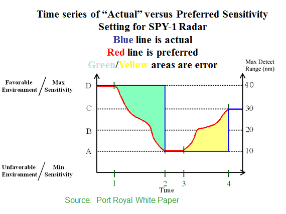 |
The letters A-D represent radar sensitivity settings. Higher sensitivity results in longer ranges (but more clutter). A favorable environment in this case means an environment with a weaker, lower, evaporation duct than in the unfavorable environment.
Let's say radar operator Joe gets on the job at time = 0. While on duty for the next two hours, the evaporation duct conditions get stronger (higher Z*) so clutter increases, making the environment for unfavorable. Although the ranges are still theoretically 40 km with this sensitivity setting, it may be more difficult to locate closer targets due to clutter increases. Finally at time = 2, Joe turns down the radar sensitivity. The range is now less, but Joe is aware of that and can now more easily find targets within the 10 nmi range of the radar at setting A. But in the period between time = 1 and time = 2, the radar was not optimally adjusted and a sudden appearing close target (e.g. submarine periscope) might be missed in all the clutter, when it could have been detected had the radar sensitivity been turned down to its optimal setting.
|
|
At time = 3, a new operator, Sam, comes on the job. Sam sees the clutter looks OK and decides to leave the radar setting as is in the low sensitivity setting. Sam didnt pay attention to evaporation duct conditions, which now trended to weaker conditions (favorable environment) as indicated by the upward moving red line. Between time = 3 and time = 4, the radar could have detected a target at a distance greater than 10 km, but was not able to because Sam never increased the sensitivity. Finally, at time = 4, Sam decides to increase the sensitivity of the radar and is able to maximize his detection range. But from the period time = 3 to time = 4 the ship was more vulnerable to attack from a cruise missile or other low-flyer than it would have been had Sam been aware of changing evaporation duct conditions.
|
|
Frequency Dependence in the Evaporation Duct |
|---|
| We showed earlier (link here to earlier module-- where is this?) how lower frequency, longer wavelength EM radiation will pass through trapping layers. This is especially important for evaporation ducts, which are much shallower than the surface-based ducts discussed in the previous module.
|
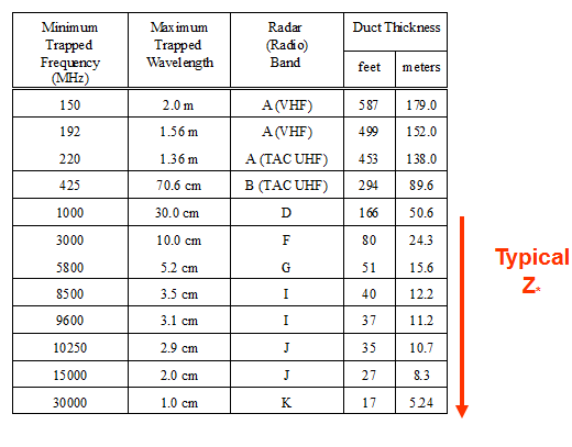
| The trapping frequency, FM, is related to the top of the evaporation duct:
Fm = 360 Z*-3/2
where Fm is the EM frequency in GHz and Z* is the height of the evaporation duct in meters.
In the table to the right, you see for typical Z* values (5 - 50 m) the lowest frequencies affected are in the 1 GHz to 30 GHz range. In order to know whether a transmission will be affected by the evaporation duct you need to know the characteristics of the duct.
|  |
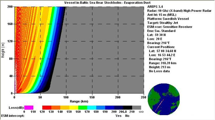
| Comparison of coverage diagrams |
| The upper image shows the AREPS coverage diagram for a standard atmosphere for a 10GHz signal with an antenna located at 10 meters above the surface.
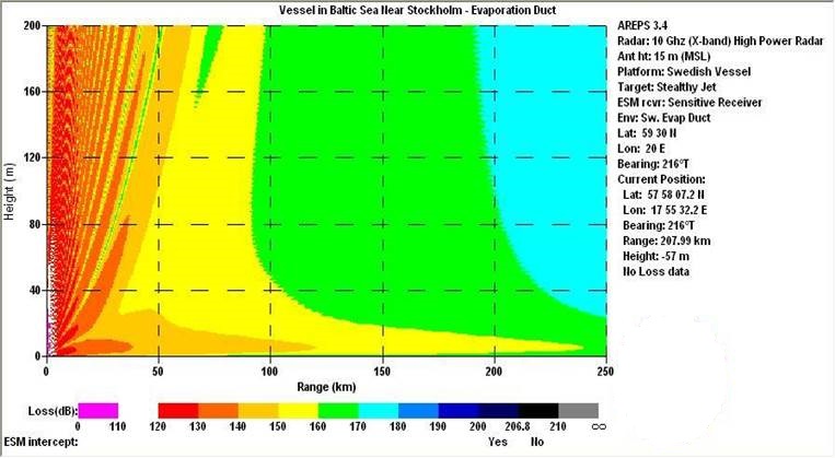
The lower image shows a similar diagram but with a 12-meter evaporation duct present. The antenna is within the duct and therefore has stronger signals and greater ranges.
|
|