| |temperature| | |salinity| | |pressure| | |density| | |dynamic_height| | |surface_height| | |velocity| |
| |temperature| | |salinity| | |pressure| | |density| | |dynamic_height| | |surface_height| | |velocity| |
Website with definitions of a number of terms used in oceanography:
http://stommel.tamu.edu/~baum/paleo/paleogloss/paleogloss.html
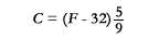
Although the rest of the world, and all scientists in the U.S. use the Celsius (previously called centigrade) scale to express ocean temperature, the equivalent values in degrees Fahrenheit are included in parentheses here since the U.S. Navy still commonly uses the Fahrenheit scale. The conversion from °Celsius (C) to °Fahrenheit (F) and vice-versa is given below.
Make sure you are comfortable working in either Celsius or Fahrenheit by using this
interactive units converter.
Temperature range in the ocean is from -2°C (28.4°F) to 30°C (86°F). In estuaries or very shallow coastal waters, temperatures could be higher. Temperature, often denoted by the symbol T, can be measured in situ using a variety of types of thermometers or thermistors. The temperature of the very thin (only microns thick) surface of the ocean, known as the skin temperature, can be measured remotely by its infrared signature. This can be done from buoys, airplanes, and satellites. The sea surface temperature is often abbreviated as SST.
The skin temperature may differ from the temperatures below, even at depths as shallow as one meter, which is as close to the surface as many in situ measurements can be made (as for example with an XBT, or CTD from a ship). Thus satellite SST measurements are adjusted to reflect the deeper "bulk" SST measurements, so that they will be consistent with the measurements made by ships.
Two physical processes contribute to this discrepancy between skin and bulk SSTs.
Temperature

Alternatively, the measured skin temperature can be cooler than the bulk temperature, although the difference is usually less than 1°C. The graph at the Met Office website: http://www.metoffice.com/research/nwp/satellite/infrared/sst/global_sst.html shows the relationship for the globally averaged SST between the bulk value and the skin value for one type of infrared instrument.
Temperature of the ocean can be changed by a heat source or sink (e.g. gaining or losing heat to the atmosphere, gaining heat from a geothermal source) or by mixing with water of other temperatures. Generally, but not always, temperature decreases with depth in the ocean.
Just as in the atmosphere, potential temperature is the temperature a parcel of water would have if it were moved adiabatically (i.e. without loss of heat) to a reference pressure. The reference pressure used for the ocean is usually the ocean surface (water pressure = 0 dbar). The potential temperature referenced to the surface will be slightly less than the in situ temperature since the expansion due to reduction in pressure leads to cooling. The symbol  is usually used for potential temperatures and the units are degrees C (or F). The numeric difference between in situ and potential temperature is almost always less than ~1.5°C, but it is important to use potential temperature when comparing temperatures of water from very different depths.
The concentration of dissolved salts in ocean water is called the salinity. While the total dissolved salts varies from place to place in the ocean due to evaporation, precipitation, river inflow, and mixing, the ratio among the various major dissolved salts remains essentially constant.
| Note: Salinity used to be expressed in terms of parts per thousand (ppt) or by weight (  ). ).
Currently, salinity is usually denoted by S and is a dimensionless quantity. |
The currently used definition of salinity was adopted when techniques to determine salinity from measurements of conductivity, temperature and pressure were developed. The UNESCO Practical Salinity Scale of 1978, PSS78, defines salinity in terms of a conductivity ratio, so is dimensionless. Therefore practical salinity is correctly written without units, although often you will see the numeric value followed by �psu� which stands for �practical salinity unit�.
Salinity may increase or decrease in depth. Open ocean salinities are generally in the range between 32 and 37, but may be much lower near freshwater sources or at the surface, and may be as high as 42 in the Red Sea.
Pressure, abbreviated p, is often used instead of depth to express the vertical coordinate in the ocean. Pressure is a function of depth, density, and gravitational acceleration.
| Pressure in the ocean is usually expressed in units of decibars, abbreviated dbar, as opposed to millibars in the atmosphere. The SI unit for pressure, kPa (kilopascals) = 103 Pa. 1 dbar = 10 kPa. |
Although the total pressure at a point in the ocean would be due both to the weight of the seawater above it and the atmospheric pressure, unless otherwise specified, the pressure at a point in the ocean is taken to be just that due to the seawater, not the seawater plus atmosphere. Therefore the sea pressure at the surface is 0 dbar. The pressure in dbar and the depth in meters are approximately equal, so the pressure in the ocean at 1 m depth is approximately 1 dbar, and that at 1000 m approximately 1000 dbar etc.
The density,  , of seawater is function of temperature, salinity, and pressure. It increases with increasing salinity and pressure, and decreases with increasing temperature. The density is expressed in units of kg/m3, or sometimes g/cm3. Oceanographers use a number of different ways to express the density of seawater, so you may see the terms density anomaly, potential density,
  (pronounced sigma-theta), specific volume, specific volume anomaly or others. The most commonly used of these are defined below.
Sigma, is a short-hand for seawater density, where 1000 kg/m3 is a short-hand for seawater density, where 1000 kg/m3has been subtracted. So for = 1024.32 kg/m3, = 24.32 kg/m3.While all the versions of have units of kg/m3, it is often reportedwithout units, which is a throwback to when the definitions included a ratio of the seawater density to the density of freshwater, thus rendering the variable dimensionless. 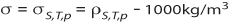 |
Sigma-t,  is density of seawater calculated with in situ salinity is density of seawater calculated with in situ salinityand temperature, but pressure equal to zero, rather than the in situ pressure and 1000 kg/m3 is subtracted. 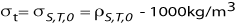 |
| Sigma-theta,
is the density calculated with in situ salinity, potential temperature, and pressure = 0, minus 1000 kg/m3.  If a pressure reference level other than the surface is used, it When comparing the density of water samples from different |
Specific volume,  , is the inverse of density; , is the inverse of density;  .
It has .
It hasdimensions of volume/mass, units of m3/kg, cm3/g, or centiliters per metric ton (cliter/ton) are usually used, where 1 cliter/ton=10-5 cm3/g. |
Specific volume (steric) anomaly,  , is the difference between , is the difference betweenthe in situ specific volume and the specific volume of seawater at the same pressure with S = 35 and T = 0°C.
The specific volume anomaly analogy to |
Dynamic height, D, is the integral of the specific volume over pressure. It is expressed in units called dynamic meters, which actually has dimensions of work per unit mass, or m2s-2. With this choice of units, the difference in dynamic height between points 1 m apart in the vertical is approximately 1 dynamic meter.
Sea surface height, usually abbreviated SSH and often denoted by the symbol  , is a measure of the difference between the actual sea surface height at any given time and place, and that which it would have if the ocean were at rest. It refers to changes in the sea surface height, or thickness of the water column from the seabed to the free surface, over horizontal spatial scales of many meters and time scales of many minutes. The SSH will be affected by tides, stratification, winds, and currents. Satellite altimeters measure the round-trip travel time of a radar pulse to estimate SSH.
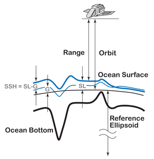
SSH = O - (R + A) - G, where O is the satellite orbital height above the reference ellipsoid; R is the range, or height, of the satellite above the sea surface; A is a correction to R due to atmospheric influences; and G is the geoid height. The geoid height is the distance between the reference ellipsoid and sea surface if the sea surface were at rest and there were no currents.
Special care must be taken when using satellite SSH measurements near coastlines. An altimeter's ground footprint, or the area over which the SSH anomaly is computed is approximately 7 km. Any footprint that includes both land and sea is contaminated, so all data within about 10 km of the coast cannot be used. Problems due to land contamination extending further out to sea occur when a satellite's track crosses from land to sea (but not the other way around). Several footprints may be affected, so SSH data within 50 km of the coast may be suspect. Also, tidal effects are removed in SSH anomaly products that are used for location of mesoscale features, so the quality of the tide model for the shelf areas of interest may affect this product.
You can learn more about measuring SSH from space at http://sealevel.jpl.nasa.gov
SSH is entirely different from significant wave height, which is a measure of the amplitude of short gravity waves on the sea surface. These gravity waves have wavelengths of only a few meters and time scales of less than a minute. Satellite altimeters can also measure significant wave height, but they use information about the character of the returned signal, rather than travel time, to do so. Some Navy products use the term "sea height" to mean significant wave height; but this could lead to confusion between significant wave height and sea surface height.
 |
|
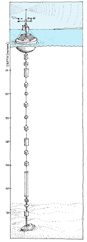
Schematic of a moored current array anchored on the ocean bottom. A buoy relays the data to a satellite. |
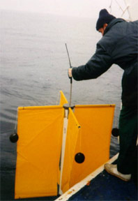
Lagrangian drifter being deployed. |
The difference between an Eulerian and a Lagrangian representation is demonstrated by the following figure:
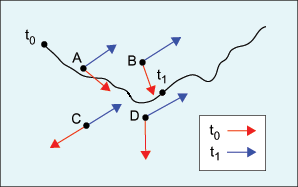
In this figure, the red arrows represent the flow at time to at fixed positions A, B, C, and D. The blue arrows represent the flow at a later time t1 at the same locations. The squiggly line represents a Lagrangian trajectory during the time period from to to t1.
Continue on to the next section in Module 1: Definitions
 ),
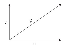
either by giving a speed and direction or by giving two perpendicular components,
for example east-west (u) and north-south (v) or along-shore and
cross-shore flow.
),
either by giving a speed and direction or by giving two perpendicular components,
for example east-west (u) and north-south (v) or along-shore and
cross-shore flow.