Upwelling Circulation on the Oregon Shelf 

(Allen, et. al.; ‘95)

LT Brady A. Brown, USN                                                                   25 Aug 2000
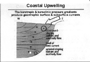Northerly winds along a western shelf force offshore flow in a turbulent surface layer.  Deep upwelling follows, as mass flux conservation fills the divergence.  Advection warps the isopycnals upward as cold bottom water rises.  A geostrophically balanced alongshore coastal jet arises.  Finally, the jet strengthens and a bottom Ekman layer carries the net water transport replacement.

The following is an analysis of a two-part experiment to model upwelling conditions across the Oregon continental Shelf found during Coastal Upwelling Experiment-2 (CUE-2) from July to August 1973. Flow fields were found to have a wide range of spatial and timescale motions.  The model used primitive-equation, 2 * layer closure, accurate bottom topography and initial density and wind conditions, on a high resolution spatial grid. 

The following variations were performed in the first part of the study:

1.Basic case (BC).

2.Double wind stress (2t_BC).

3.Add heat flux (Q).

4.Reduce density field by * (0.5 N²_BC).

5.Reduce density field by * (0.25 N²_BC).

6.Homogeneous case (N² = 0).

7.Wide shelf topography (Wide).

8.Steep shelf topography (Steep).

9.Sheer vertical shelf (Vertical).

10.Vertical turbulent kinematic viscosity constant (K_M = K_H = 0.0005 m²/s).

11.As above & diffusivity a function of Richardson number (K_M, K_H (R_i  PP*)).

12.As above & diffusivity a function of Richardson number (K_M, K_H (R_i  HR**)).

13.Grid refined (Dx = 0.25 km).

14.Grid refined (Dx = 0.166 km).

15.Grid expanded (x = 200 km).

 *   Pacanowski & Philander (1981) parameter dependency equation.

 ** Hamilton & Rattray (1978) [based on Munk & Anderson (1948)].

For the second study, the following variable were adjusted:

16.Base heat flux (Q = 166 W/m²).

17.No heat flux (NQ).

18.Add pressure gradient (Q+P_y = -3.9₁₀^-7 m/s²).

19.Initial state of rest (Q_ifi).

20.Double heat flux (2Q).

21.Low-pass filtered wind stress (Q_t/p).

22.Shore wind stress applied (Q_t/Newport).

23.Curl of wind stress computed (Q_Ñxt).

Observed behaviors were successfully shown by the model results.  Most of the upwelling took place in a shallow surface layer, density gradients steepened, and the offshore edge of the frontal jet produced high turbulent energy values at about 4 km offshore and 30 meters depth, which then translated offshore at about * km/day.

The two-dimensional analysis that followed showed all expected features, but time-dependent oscillations arose after day 16 below the upwelling front that were longer than inertial in timescale; “...further research is required to determine the dependence of this behavior on the turbulence submodel...”.  Also, three-dimensional assumptions must be made to track coastal jet mass transport as this has a great effect on heat flux parameters.

 

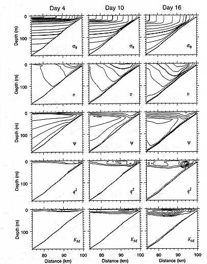Figure 1.  Basic case density field, along-shore velocity, across-shelf streamfunction, turbulent kinetic energy, and vertical kinematic viscosity.

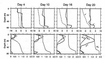
Figure 2. Vertical profiles at 60m isobath (about 8 km offshore).

The most important aspects of these characteristic changes include:

üDouble winds produced velocity fields in half the model time.

üHeat flux deepened surface mixed layer and drove jet further offshore.

üReduced density increased bottom layer and Rossby radius, and less velocity.

üHomogeneous case had no jet flow, and double Rossby radius.

üSteep shelf made friction less effective; geostrophic balance affected.

üViscosity increase lowered streamflows and eliminated oscillations.

üSmaller grid had no effect; larger size means faster computations.

üChanging heat flux had no effect below about 40m.

üModel surface layer too large (25m); lower 19m time-varying depth average used.

üWind changes not as important as topography.

Allen, J.S., P.A. Newberger, and J. Federiuk, 1995: “Upwelling Circulation on the Oregon Continental Shelf.  Part I: Response to Idealized Forcing.”  American Meteorological Society, Vol. 25, 1843-1866.

Chu, Peter, 2000.  Naval Postgraduate School, Monterey, CA.  Lecture review, OC4331: Prediction of Naval Models.

Federiuk, J., and J.S. Allen, 1995: “Upwelling Circulation on the Oregon Continental Shelf.  Part II:Simulations and Comparisons with Observations.”  American Meteorological Society, Vol. 25, 1867-1889.

www.epic.noaa.gov      Historical climatological database.

www.es.umb.edu         Online oceanography course material.
 

This is a government-maintained internet site. Please read the U.S. Navy web page disclaimerand the disclaimer regarding external links.