Lab10: Variability of Atmospheric Forcing

The link between the atmosphere and the ocean consists of thermal
and momentum fluxes across the air/sea interface. For numerical
models these fluxes are calculated based on long and short wave
radiation, air temperature, sea surface temperature, wind, vapor
pressure, and precipitation. There are some public source for the
atmospheric facing, some sources avalible on web site, and some
on CD that you can order. In this lab, we will learn how to get
some get the data from NetCDF (network Common Data Form) data.

There are some public data source such as:

International Comprehensive Ocean-Atmosphere Data Set (ICOADS). http://icoads.noaa.gov/

National Centers for Environmental Prediction (NCEP) Data set. http://www.ncep.noaa.gov/

National Snow and Ice Data Center http://nsidc.org/data/nsidc-0057.html

The data sets can be download as the Netcdf format.

What is NetCDF data format?

NetCDF (network Common Data Form) is an interface for array-oriented
data access and a freely-distributed collection of software libraries
for C, Fortran, C++, Java, and perl that provide implementations of
the interface. The netCDF software was developed by Glenn Davis,
Russ Rew, Steve Emmerson, John Caron, and Harvey Davies at the
Unidata Program Center in Boulder, Colorado, and augmented by
contributions from other netCDF users. The netCDF libraries define
a machine-independent format for representing scientific data.
Together, the interface, libraries, and format support the creation,
access, and sharing of scientific data.

NetCDF are not standard Matlab library, it is necessary to install the NetCDF library and some application code to make Matlab can work on NetCDF file.

Why we like NetCDF data?
1. machine-independent
2. the data installed as binary, so to access is very fast and
get the part of the data directly.
3. as it is a structure (or CELL in matlab), beside the data,
it also contain a lot of information about the data, such
as: what is the data, units, data region, fact, off_set,......
4. it also can install the data as a short integer binary data
(2 bit) instead of real number(4 bit). Make the size even small.

PROCEDURE

Note: NetCDF format is not the

copy lab10 director and netcdf interface files to your director as:

Click \\Lrcapps\common$\OC4323, copy Lab10 folder to your os4323 directory.

Click \\Lrcapps\common$\OC4323, open matlabXXX folder (for tour matlab version) then copy adnetcdfRxxx.m and netcdfRxxx.dll to your Lab10 folder. Change the file name to adnetcdf,m and netcdf.dll.

Open matlab program than change current folder to oc4323/Lab10.

Down load monthly mean air temperature and Scalar Wind NetCDF data from ICOADS Data set

Click on ICOADS web set http://icoads.noaa.gov/

ð Click on Data and Metadata => click on Access statistics in netCDF format (1991-) => click on air.mean.nc to download this netcdf data and save on your work space (Lab10).

ð Back to Data and Metadata web site => click on Access options from PSD in netCDF format => click on ICOADS 2°x2° products (1800-Dec 2007) => click on Scalar Wind (w) wapd*.nc => click on Monthly Mean wspd.mean.nc to download the monthly mean scalar wind data and save it.

View the netcdf data:
>> adnetcdf;


(1) View NetCDF data:

a. view monthly mean air temperature netcdf data:

>> ncbrowser air.mean.nc nowrite (or ncbrowser('air.mean.nc','nowrite') )

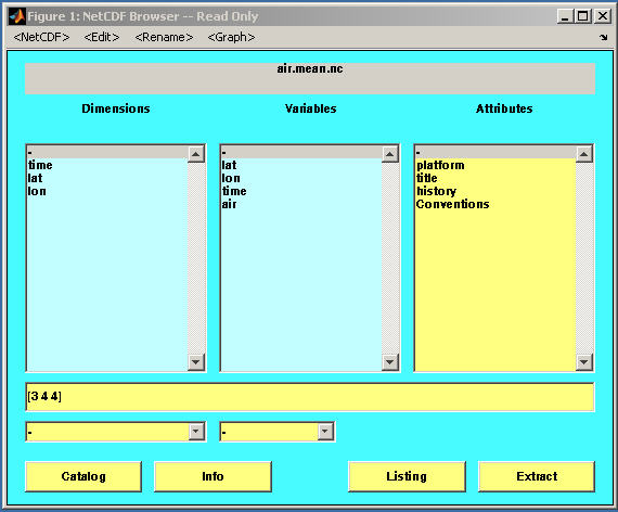
A Netcdf data structure browser will open. You can see all the information about this data structure. There are three parts: data dimensions, Variables and Attributes. You can click on each one to see the detail information.

Click on variables lat, this is one dimension array with dimension 90 (lat) and the data type is float (real number). Then click on the long_name (Attributes) the name of lat will listed.

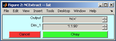
Click on variables lat again, then click on the listing (bottom line), the value of lat will listed on your matlab domain. (Note: the listing only list the values but will not be stored in variable). If you like load the variable (lat), click lat, then click Extract, a extract window will open, the default output variable name is ncx (you can change to other name), click on Okey to load the values of lat. You also can load part of the variable by change the dimension region.

Close all the window

>> close all;

b. view monthly mean scalar wind netcdf data:

>> ncbrowser('wspd.mean.nc','nowrite');

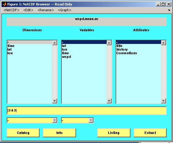
Click on lat,lon,time (variables), you can see all these three variables are Coordinate variables with the data type float (single real number) and double (double real number).

Click on wspd (variables), it is variable and with data type short (integer*2 or short integer: with range: -32767 – 32766). Check the missing_value, add_offset and scale_factor on the Attributes, the values are: 32766, 327.65 and 0.01. That mean the data wspd store in the netcdf file as the short format instead of float to save the data storage. Any value as 32766 indicated the missing value, and the others will be integer value (not the real value). You must convert the integer value to the real number as real_value = integer_value*scale_factor + add_offset.

Click on wspd again (variables), the dimensions show [2496, 90, 180], and in the Dimensions window list the name as time,lat,lon. That mean the dimension ordered as [time,lat,lon].

To load wspd:

Click Extract button:

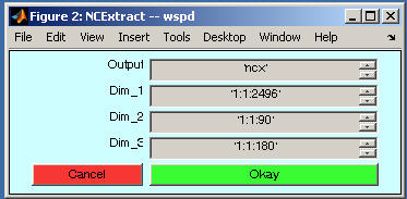
If you like to load part of the data, just modify the number in the Dim_*, then click Okey. Be careful, as the original wspd is real number but store as integer number, it must be converted. It can be:

>> ii=find(ncx==32766); % find any missing value index

>> ncx(ii)=NaN; % set missing value as NaN

>> wspd = ncx * 0.01 + 327.65;

(2) Load data from netcdf file in program:

Even ncbrowser can be used to load Netcdf data, but it is not convenience to be used in the matlab program. There are some application code such as netrcdf and snctools can be used to programming the matlab code.

The follow we will discuss how netcdf code works.

a. load wspd data from wspd.mean.nc

>> nc=netcdf('wspd.mean.nc','nowrite'); % open a netcdf file as a structure

>> ofst=nc{'wspd'}.add_offset(:); % get add_offset value

>> fact=nc{'wspd'}.scale_factor(:); % get scale_factor value

>> wspd=nc{'wspd'}(:); % load all the wspd data

>> ii=find(wspd==32766); % find missing value index

>> wspd(ii)=NaN; % set the missing value to NaN

>> wspd=wspd*fact+ofst; % convert the integer to real number

>> nc=close(nc); % close netcdf file

b. load part of air temperature data from air.mean.nc

load 2004 May Pacific Ocean Air temperature data. (lon: 120E ~ 210E , lat: 40S – 60N)

Use ncbrowser to view the data structure in this netcdf file.

>> ncbrowser air.mean.nc nowrite;

The data we want to load is part of variable air. Check the air, it is a 3-D data with the dimension [time,lat,lon]. You have to figure out what is the index region for each dimension.

>> nc=netcdf('air.mean.nc','nowrite');

>> time=nc{'time'}(:);

>> lat=nc{'lat'}(:);

>> lon=nc{'lon'}(:);

>> missval=nc{'air'}.missing_value(:); % get the air missing value

After you load all the Coordinate variables, you have to figure out the time index, latitude and longitude index region for the 2004 May pacific ocean region.

There are two ways to get the time index for 2004 May. As this data temporal coverage is: Monthly values for 1991/01 – present. So the index for 2004 May should be: 12*(2004-1991)+5=161. The another way to determine the time index is to convert the julian day to year month and day, than find the correct index.

>> refjday=ymd2jday(1991,1,15); % find the julian day for 1991/1/15

>> [year,month,day]=jday2ymd(time+refjday-time(1)); % convert the julian day to year month and day

>> itime=find(year==2004 & month==5); % find the time index for 2004 May

To find latitude index can be:

>> [mmm,ilat1]=min(abs(lat-60)); % find the index to close 60

>> [mmm,ilat2]=min(abs(lat-(-40))); % find the index to close -40

Same way to find longitude index region as:

>> [mmm,ilon1]=min(abs(lon-120));

>> [mmm,ilon2]=min(abs(lon-210));

Now you can load the air temperature data exact for 2004 May Pacific Ocean as:

>> airtemp=nc{'air'}(itime,ilat1:ilat2,ilon1:ilon2);

>> nc=close(nc);

>> ii=find(airtemp==missval);

>> airtemp(ii)=NaN;

>> lonn=lon(ilon1:ilon2);

>> latt=lat(ilat1:ilat2);

>> contour(lonn,latt,airtemp);

>> hold on;

>> lonw=min(lonn); lone=max(lonn); lats=min(latt); latn=max(latt);

>> [xcoast,ycoast]=getcoastline(lonw,lone,lats,latn);

>> plot(xcoast,ycoast,'g','linewidth',2);

>> set(gca,'xlim',[lonw,lone],'ylim',[lats,latn]);

>> xlabel('Longitude');

>> ylabel('Latitude');

>> title('Air Temperature (Pacific Ocean)');

c. load air temperature data for 2005 Aug South Atlantic Ocean from air.mean.nc

Region: latitude: 80S -0, longitude 70W – 20E.

Note: As the longitude for this data is from 0 – 359, so you have to load the data in two parts. One is from 70W - 1W (or 290 – 359), the another part is from 0E – 20E. Then combine the two parts to one data using cat function.

Turn in:

Contour plot 2005 Aug South Atlantic air temperature data, save as jpeg file and email to: fan@nps.edu