Naval Postgraduate School OC3902

FUNDAMENTALS OF MAPPING, CHARTING, AND GEODESY

LABORATORY 7

Map Projections (Matlab Version.7)

Objectives

A. Use MATLAB mapping database with MATLAB mapping toolbox to create different map projections.

B. Use your own high resolution coastlines data to create map projections with MATLAB mapping toolbox.

C. Use MATLAB to make a Geographic (plate Carree) map projection without MATLAB mapping toolbox.

References

DMA Manual DMA-TM-8358.1.Datums, Ellipsoids, Grids and Grid Reference Systems.

Snyder, J.P., (1987).Map Projections - A Working Manual.US Geological Survey Professional Paper 1395.

MATLAB mapping toolbox.

Background

Maps and, by implication, map projections are essential to military operations. Nearly all the tactical decisions for positioning military assets are made with respect to either a map or a set of coordinates. The ability to correctly interpret such data is an essential part of any military operation.

This lab will be broken into three parts designed to highlight the key objectives outlined above.

Copy lab7_map to your local workspace from \\lrcapps\common$\OC3902\FY09Qtr1\ .

Or down load CTD station data CTDST.txt and topography data for PC topo.mat or topography data for Linux topounix.mat, or netcdf data topography data topo.nc.

An Introduction to Mapping Toolbox

The Mapping Toolbox provides a comprehensive set of functions and graphical user interfaces for building map displays and performing geospatial data analysis in MATLAB. You can create map displays that combine data from multiple modalities and display them in their correct spatial relationships. The toolbox supports standard analyses, such as line-of-sight calculations on terrain data or geographic computations that account for the curvature of the Earth's surface. Most of the functions in the Mapping Toolbox are written in the open MATLAB language. This means that you can inspect the algorithms, modify the source code, create your own custom functions, and automate frequently performed tasks.

The toolbox supports key mapping and geospatial data analysis, manipulation, and visualization tasks that are useful in applications such as earth and planetary scientific research, oil and gas exploration, environmental monitoring, insurance risk management, aerospace, defense, and security.

The Mapping Toolbox allows you to read, analyze, and display geographic information within MATLAB. Since the earth and most heavenly bodies are generally spherical in shape, geographic data is usually defined on a spherical or elliptical coordinate system. Distance, azimuth, area, and even straight lines on the curved surface of the earth are defined differently than in the MATLAB Cartesian coordinates. Displaying geographic data from round bodies on flat surfaces also requires special techniques from the art of cartography. The Mapping Toolbox can create maps using simple commands that make reasonable cartographic choices or allow you to control every detail of the map display. Atlas data provided with the toolbox allows you to create detailed base maps on which you can plot your own results. You can also import high-resolution map data available over the Internet from government or academic sources.

Geographic data is usually displayed on a base map containing features like coastlines or topography. The first step in the preparation of a base map is the selection of an appropriate projection. Projections are ways of representing features from a round body on a flat piece of paper or computer screen. The art of displaying a three-dimensional body on a two-dimensional surface is called cartography. Cartographers have devised many different projections, each a different compromise between fidelity of scale, shape, and direction. The art in cartography is partly the selection of a projection that is appropriate to the task at hand.

Note: As the map created by MATLAB mapping toolbox is different than MATLAB Cartesian coordinates, some original MATLAB function (such as plot, line, patch, contour) can no longer be used; instead use plotm, linem, patchm and contourm. Use help command to see the detailed information on these commands.

The most advantage of Mapping tool version 7 is now it support shapefile (see shaperead).

There are two auto map projection functions worldmap and usamap to automatic define the map projection, the frame(framem), the grid(gridm), and the meridian(mlabel) and the parallel(plabel) labels on the map axes.

You also can define the map projection by yourself use axesm.

Part A: Use MATLAB mapping database with MATLAB World map projection (worldmap)

Example1: world map (line only)

>> worldmap('world');

>> load coast;

>> plotm(lat,long);

Note: plotm is similar as plot, but input variables must y first x second.

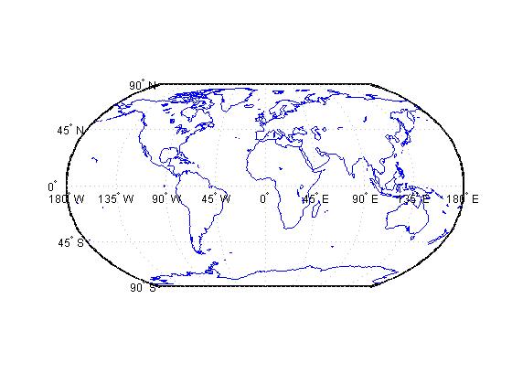
If you like to change the projection

>> axesm;

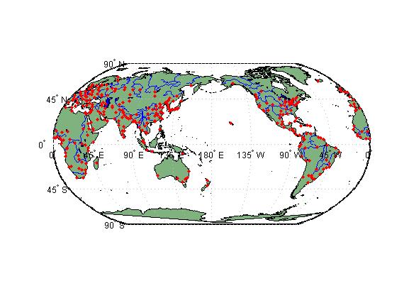
Example2: worldmap with land areas, major lakes and rivers, and cities and populated places:

>> ax=worldmap('world');

>> setm(ax,'Origin',[0,180,0]); %[ latitude longitude orientation]

>> land = shaperead('landareas', 'UseGeoCoords', true);

>> Hd=geoshow(ax, land, 'FaceColor', [0.5 0.7 0.5]);

>> lakes = shaperead('worldlakes', 'UseGeoCoords', true);

>> Hk=geoshow(lakes, 'FaceColor', 'blue');

>> rivers = shaperead('worldrivers', 'UseGeoCoords', true);

>> Hr=geoshow(rivers, 'Color', 'blue');

>> cities = shaperead('worldcities', 'UseGeoCoords', true);

>> Hc=geoshow(cities, 'Marker', '.', 'Color', 'red');

>> tightmap;

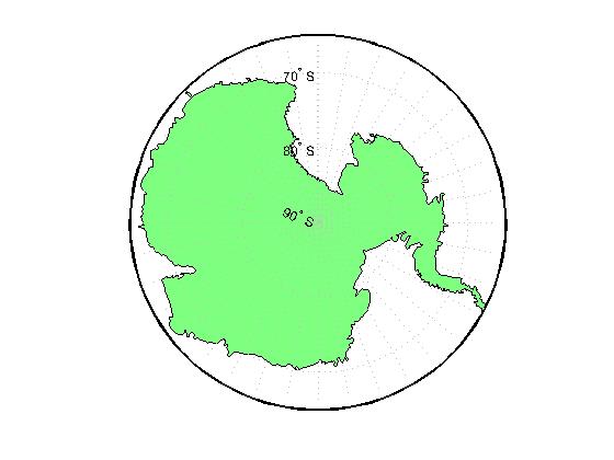
Example3: Draw a map from exist region name.

If you don’t know the region name:

>> worldmap;

Than select the region name.

If you know the region name you can input the region name as:

>> worldmap(' antarctica');

>> antarctica = shaperead('landareas', 'UseGeoCoords', true,'Selector',{@(name) strcmp(name,'Antarctica'), 'Name'});

>> patchm(antarctica.Lat, antarctica.Lon, [0.5 1 0.5]);

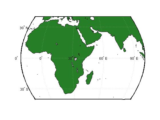
You also can input multi region names in one map as:

>> worldmap ({'Africa','India'});

>> land = shaperead('landareas.shp', 'UseGeoCoords', true);

>> geoshow(land, 'FaceColor', [0.15 0.5 0.15]);

Example4: Draw a map from latitude and longitude region

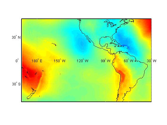
>> worldmap([-50 50],[160 -30]);

>> load geoid;

>> Hg=geoshow(geoid, geoidrefvec, 'DisplayType', 'texturemap');

>> load coast;

>> Hl=geoshow(lat, long);

Question: 1. What is the current map projection?

2. Can you move the meridian labels from canter to bottom?

3. Can you change to map projection “plate carree”?

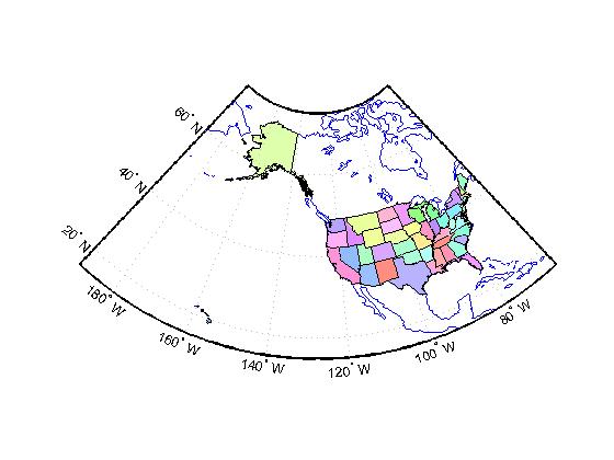
Example5:

>> ax = worldmap('USA');

>> load coast

>> plotm(lat, long);

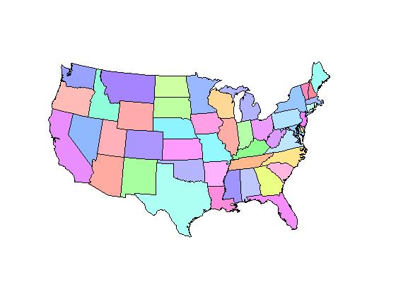
>> states = shaperead('usastatelo', 'UseGeoCoords', true);

>> for k = 1:numel(states)

states(k).Number = k;

end

>> faceColors = makesymbolspec('Polygon',{'Number', [1 numel(states)], 'FaceColor', polcmap(numel(states))});

>> Hs=geoshow(ax, states, 'DisplayType', 'polygon', 'SymbolSpec', faceColors);

Part B: MATLAB USA Map Projection (usamap)

USAMAP Construct a map axes for the United States of America.

USAMAP STATE or USAMAP(STATE) constructs an empty map axes with a Lambert Conformal Conic projection and map limits covering a U.S. state or group of states specified by input STATE. STATE may be a string or a cell array of strings, where each string contains the name of a state or 'District of Columbia'. Alternatively, STATE may be a standard two-letter U.S. Postal Service abbreviation. The map axes is created in the current axes and the axis limits are set tight around the map frame.

usamap 'conus' or usamap('conus') constructs an empty map axes for the conterminous 48 states (i.e. excluding Alaska and Hawaii).

usamap with no arguments asks you to choose from a menu of state names plus 'District of Columbia', 'conus', 'all', and 'allequal'.

usamap(latlim, lonlim) constructs an empty Lambert Conformal map axes for a region of the U.S. defined by its latitude and longitude limits in degrees. latlim and lonlim are two-element vectors of the form [southern_limit northern_limit] and [western_limit eastern_limit], respectively.

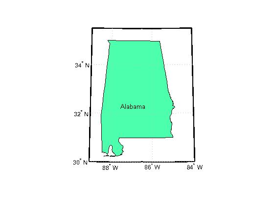
Example6: map for one state

>> figure; ax=usamap('Alabama');

>> alabamahi = shaperead('usastatehi', 'UseGeoCoords', true,'Selector',{@(name) strcmpi(name,'Alabama'), 'Name'});

>> geoshow(alabamahi, 'FaceColor', [0.3 1.0, 0.675])

>> textm(alabamahi.LabelLat, alabamahi.LabelLon, alabamahi.Name,'HorizontalAlignment', 'center');

>> setm(ax,'MapLatLimit',[30,35.5],'MapLonLimit',[-89,-84]);

Example7: map for multi states

>> figure;

>> ax = usamap({'CA','MT'});

>>% or ax=usamap([30,50],[-126,-103]);

>> latlim = getm(ax, 'MapLatLimit');

>> lonlim = getm(ax, 'MapLonLimit');

>> states = shaperead('usastatehi','UseGeoCoords', true, 'BoundingBox', [lonlim', latlim']);

>> geoshow(ax, states, 'FaceColor', [0.5 0.5 1])

>> for k = 1:numel(states)

labelPointIsWithinLimits =latlim(1) < states(k).LabelLat && latlim(2) > states(k).LabelLat && lonlim(1) < states(k).LabelLon && lonlim(2) > states(k).LabelLon;

if labelPointIsWithinLimits

textm(states(k).LabelLat,states(k).LabelLon, states(k).Name,'HorizontalAlignment', 'center')

end

end

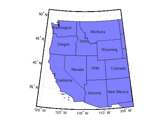
Try use the latitude and longitude region instead of state names.

Example8: Map the Conterminous United States with a different fill color for each state

>> figure; ax = usamap('conus');

>> states = shaperead('usastatelo', 'UseGeoCoords', true,'Selector',{@(name) ~any(strcmp(name,{'Alaska','Hawaii'})), 'Name'});

>> for k = 1:numel(states)

states(k).Number = k;

end

>> faceColors = makesymbolspec('Polygon',{'Number', [1 numel(states)], 'FaceColor',polcmap(numel(states))});

>> geoshow(ax, states, 'DisplayType', 'polygon','SymbolSpec', faceColors);

>> framem off; gridm off; mlabel off; plabel off

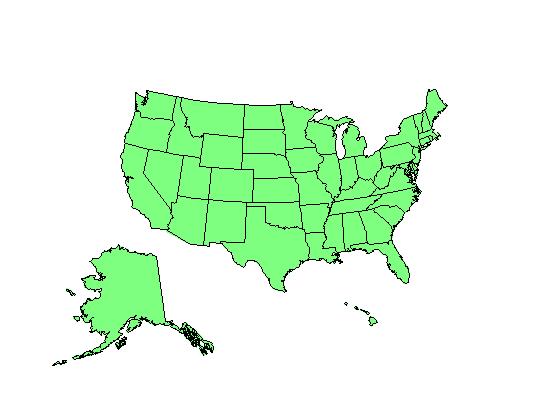
Example9: Map of the USA with separate axes for Alaska and Hawaii:

>> figure; ax = usamap('allequal');

>> states = shaperead('usastatelo', 'UseGeoCoords', true);

>> names = {states.Name};

>> indexHawaii = strmatch('Hawaii',names);

>> indexAlaska = strmatch('Alaska',names);

>> indexConus = 1:numel(states);

>> indexConus(indexHawaii) = [];

>> indexConus(indexAlaska) = [];

>> stateColor = [0.5 1 0.5];

>> geoshow(ax(1), states(indexConus), 'FaceColor', stateColor)

>> geoshow(ax(2), states(indexAlaska), 'FaceColor', stateColor)

>> geoshow(ax(3), states(indexHawaii), 'FaceColor', stateColor)

>> for k = 1:3

setm(ax(k), 'Frame', 'off', 'Grid', 'off','ParallelLabel', 'off', 'MeridianLabel', 'off');

end

Part C: Define map axes and set map properties (axesm)

The axesm function creates a map axes object complete with a map data structure. Maps must be displayed in map axes. All standard MATLAB axes properties of map axes are controlled by the axes function, along with set and get. Map axes properties are defined on creation with axesm and can be queried and changed after creation of a map axes using getm and setm.

axesm with no input arguments, initiates the map axes graphical user interface, which can be used to set map axes properties. All the map projections and properties can be selected by “windows” and it is much easy to make the right map projection and all the properties that you wish.

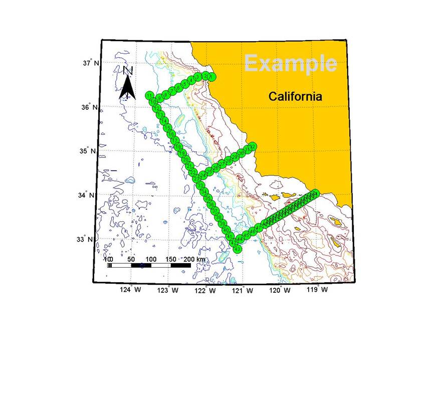
Example10: Draw a map for CDT data (as Lab4), the map will be:

a. Map projection: Lambert Conformal Conic. With Latitude: 32N – 37.3N, Longitude: 125W – 118W.

b. Draw California land map.

c. Draw Ocean Depth contours. (load topo.mat)

d. Marker the CDT station locations with ID number. (load CDTST.txt)

e. Make a North Arrow on the map.

f. Make a Scale Ruler on the map

Procedure:

a. Map projection: Lambert Conformal Conic. With Latitude: 32N – 37.3N, Longitude: 125W – 118W

>> figure('units','inches','position',[1,2.5,8,7]);

>> axes('position',[0.05,0.05,0.9,0.9]);

>> xlm=[-125,-118]; ylm=[32,37.3];

>> axesm; % Will open the Projection Control window and fill what you want.

Map Projection: Coni: Lambert Conformal Conic

Map Limits: Latitude 32 37.3 Longitude -125 -118

Map Origin: lat 0 lon -121.5 orientation 0

Frame Limits: Latitude 32 37.3 Longitude -3.5 3.5

Parallels: 36.5 33

Click frame, Grid, Labels to define the frame, grid and labels.

b. Draw California land map.

>> land=shaperead('usastatehi','UseGeoCoords', true,'BoundingBox',[-125,32;-118,37.3],'Selector',{@(name) strcmpi(name,'California'), 'Name'});

>> geoshow(land, 'FaceColor', [1,0.8,0]);

>> disp(['Click for the State Name center position']);

>> [ylat,xlon]=inputm(1);

>> textm(ylat, xlon, land.Name,'HorizontalAlignment','center','fontsize',16,'fontweight','demi');

c. Draw Ocean Depth contours. (load topo.mat)

>> load topo.mat;

>> contourm(latt,lonn,topo,-[500:500:4500]);

d. Marker the CDT station locations with ID number. (load CDTST.txt)

>> load CTDST.txt;

>> plotm(CTDST(:,3),CTDST(:,2),'o','MarkerEdgeColor','k','MarkerFaceColor','g','Markersize',12);

>> for k=1:size(CTDST,1)

textm(CTDST(k,3),CTDST(k,2),int2str(CTDST(k,1)),'HorizontalAlignment', 'center','fontsize',6);

end

e. Make a North Arrow on the map.

>> disp(['Click for the NorthArrow Position (Arrow Tail)']);

>> [yy,xx]=inputm(1);

>> northarrow('latitude',yy, 'longitude',xx);

f. Make a Scale Ruler on the map

>> disp(['Click for the ScaleRuler Position (start position)']);

>> [xx,yy]=ginput(1);

>> scaleruler('Xloc',xx,'Yloc',yy,'MajorTickLength',10,'MajorTick', 0:50:200,'RulerStyle', 'patches');

>> hidem(gca); % or axis('off');

Rurn in:

Save the CDT Stations map as jpg file and email to: fan@nps.navy.mil

  (Back to "Labs List" page.)

Last Updated 29 Sept. 2008
POC: Peter Chu