OC3140
Lab 9 Linear Regression
1
Objectives
In this lab, you use the
linear regression to find the relationship between Mixed Layer Depth and Sea
Surface Temperature in the
2
Procedure
A. Data Preparation
·
Make a folder for lab9
in your local director and download the data MixDepSST.mat
from \\lrcapps\common$\OC3140\lab9.
·
Start matlab
and change the work space to your oc3140 lab9 directory.
·
Load the Mixed
Layer Depth (mixdep) and Sea Surface Temperature (sst)
data
>>
load
MixDepSST;
·
Set sst
-> x, and mixdep->y
>> x=sst; y=mixdep; n=length(x);
·
Determine the regression
coefficients (see Ch9):

>> xmean=mean(x);
ymean=mean(y);
% mean variable ![]()
>> Sxx=sum(x.^2)-sum(x)^2/n;
>> Syy=sum(y.^2)-sum(y)^2/n;
>> Sxy=sum(x.*y)-sum(x)*sum(y)/n;
>> b1=Sxy/Sxx; b0=ymean-b1*xmean;
·
Residual Analysis (see Ch9):
![]()
>> yy=b0+b1*x; % the predicted ![]()
>> er=y-yy;
% the error ![]()
>> Se2=sum(er.^2)/(n-2);
% sample variance
(or Se2=(Syy-b1*Sxy)/(n-2);
)
>> Se=sqrt(Se2);
·
Analysis of Variance
(AVOVA) (see Ch9):

>> SSR=sum((yy-ymean).^2); % The Regression Sum of Square
>> SSE=sum((y-yy).^2); % Sum of Squared Error
>>
SST=SSE+SSR; % Total Sum of Squares
>> MSR=SSR;
MSE=SSE/(n-2);
% Mean Regression of Square and Mean Squared Error
>> F=MSR/MSE; % F statistic
value
·
Goodness-of-fit Measures
(see Ch9):

>> MSE=Se2; % Mean
Squared Error (MSE)
>>
R2=SSR/SST;
% Coefficient of determination (R^2)
·
Confidence Intervals:
Base on ![]() (see Ch9):
(see Ch9):
A ![]() confidence interval
for the regression coefficient
confidence interval
for the regression coefficient ![]() is
is

A ![]() confidence interval
for the regression coefficient
confidence interval
for the regression coefficient ![]() is
is
![]()
A ![]() prediction interval
for individual predicted values is
prediction interval
for individual predicted values is

(a). Confidence Interval for Regression
Coefficient (b0 and b1):
>> bint0=b0+1.96*sqrt(sum(x.^2)/(n*Sxx))*Se*[-1,1];
>>
bint1=b1+1.96*Se/sqrt(Sxx)*[-1,1];
(b). Prediction
Interval of ![]()
>> yyint=yy*ones(1,2)+1.96*sqrt(1+1/n+(x-xmean).^2/Sxx)*Se*[-1,1];
B.
Comparison between your
results and the Matlab function regress
·
A matlab
function regress.m can be used to calculate multiple
linear regress. Learn how to use regress function from >> help regress, or open help Navigator.
REGRESS Multiple linear regression
using least squares.
b = REGRESS(y,X) returns the vector of
regression coefficients, b,
in
the linear model y = Xb,
(X is an n*p matrix, y is the n*1
vector
of observations).
[B,BINT,R,RINT,STATS] = REGRESS(y,X,alpha) uses the input, ALPHA
to
calculate 100(1 - ALPHA) confidence intervals for B and the
residual vector,
R, in BINT and RINT respectively. The default value of
alpha is 0.05.
The vector STATS contains the R-square statistic along with
the
F and p values for the regression.
The X matrix
should include a column of ones so that the model
contains
a constant term. The F and p values are
computed under
the
assumption that the model contains a constant term, and they
are
not correct for models without a constant.
The R-square
value
is the ratio of the regression sum of squares to the
total sum of
squares.
·
Create a matrix for the
independent variable. In order to
properly calculate the slope and intercept with regress (below), this matrix must have a column of 1's and a
second column that contains the independent variable. The following command, for example, will
construct an independent variable matrix, sst2, for the variable sst.
>> sst2 = [ones(size(sst)),
sst];
·
Perform the regression
to generate the equation between the mixdep and the
corresponding sst using matlab function regress.
>> [b,bint,r,rint,stats]
= regress(mixdep,sst2);
This function gives you the slope (b(2)) and intercept (b(1)) values, the 95% confidence
intervals for the slope (bint(2,:))
and intercept (bint(1,:)), the residuals (r) and the error bounds on each
residual value (rint). The three-element vector stats contains the
"r-squared" value (stats(1)),
the F-statistic (stats(2)),
and the p-value (stats(3)). The "r-squared" value will be
useful to you: it is just the square of the correlation coefficient for this
data. Recall that a large correlation
coefficient implies that your data sets have a fairly linear relationship. We will not be concerned with the F-statistic
or the p-value in this lab.
·
Compare the follow data that you
prepared with the result of matlab function regress:
Prepared
data function
regress result
b0 b(1)
b1 b(2)
bint0 bint(1,:)
bint1 bint(2,:)
R2 stats(1)
F stats(2)
·
Comparison Data in the table:
Comparison Table
|
|
Prepared data |
From function regress |
|
Intercept value |
69.6844 |
69.6844 |
|
slope |
-1.667 |
-1.667 |
|
95% confidence intervals for
intercept |
[64.0455, 75.3233] |
[64.0283, 75.3415] |
|
95% confidence intervals for slope |
[-1.8573, -1.4767] |
[-1.8579, -1.4761] |
|
Coefficient of determination |
0.4416 |
0.4416 |
|
F-statistic |
294.9318 |
294.9318 |
C.
Plot
·
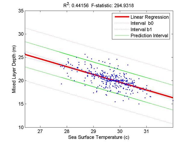
Plot the regression line, confidence
intervals for regression coefficients and prediction interval of ![]() , and produce a "scatter plot" for the pair of data,
and static information on one figure.
, and produce a "scatter plot" for the pair of data,
and static information on one figure.
>>
figure;
>> xlm=[min(sst),max(sst)];
>> set(gca,'xlim',xlm,'box','on'); hold on;
>> plot(xlm,b0+b1*xlm,'r-','linewidth',3); % regression line
>> plot(xlm,bint0(1)+b1*xlm,'r:'); %
one of interval b0
>> plot(xlm,ymean+(xlm-xmean)*bint1(1),'b:');
% one of interval b1
>> plot(sst*[1,1],yyint,'g'); %
prediction interval
>> plot(xlm,bint0(2)+b1*xlm,'r:'); %
another interval b0
>> plot(xlm,ymean+(xlm-xmean)*bint1(2),'b:');
% another interval b1
>> plot(sst,mixdep,'.'); %
scatter plot for data
>> legend('Linear
Regression','Interval
b0','Interval b1','Prediction Interval');
>> xlabel('Sea Surface
Temperature (c)');
>> ylabel('Mixed Layer Depth
(m)');
>> title(['R^2:
',num2str(R2),' F-statistic:
',num2str(F)]);
>> print
–djpeg lab9;
3 Turn in: No requirement