The choice of a vertical coordinate system is one of the most important aspects of a
model's design.
There are three main vertical coordinate systems in use.
Each one has its advantages and disadvantages, which has led to the development of
hybrid coordinate systems. This is an area of very active research and development in numerical
ocean models.
The following discussion follows Chassignet et al., 2002.
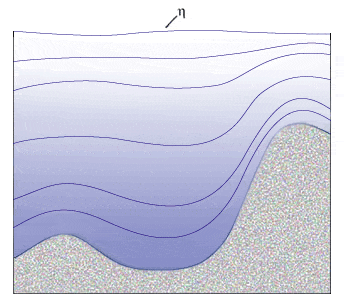
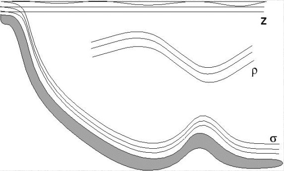
- z-coordinates. In this coordinate system, the vertical coordinate is depth, or "z".
This system is the simplest and has been in use in various ocean models for decades.
z-coordinate models excel in areas that are well-mixed because they can provide
the very fine resolution needed to represent three-dimensional turbulent processes.
There are a fixed number of depth levels in the ocean, and these can be placed to give
higher resolution in the surface layer where it is needed the most.
Where z-coordinates have a disadvantage is in regions of sloping topography -
here the levels intersect the bathymetry and unrealistic vertical velocities
near the bottom can result.
Increasing the number of vertical levels will improve the representation
of the near-bottom flow, but at a high computational cost.
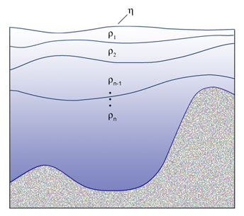
- sigma (
 )-coordinates.
In this type of model, the vertical coordinate follows the bathymetry,
keeping the same number of vertical grid points
everywhere in the domain, no matter how deep the water column.
The layer thicknesses vary from horizontal grid point to grid point as the bottom depth
varies.
The sigma-levels do not have to be
evenly distributed over the water column.
Often they are more closely spaced near the surface and/or bottom
than in the interior, thus allowing the boundary layers
to be better resolved everywhere in the domain.
This could not be done with a z-level model without an excessively large number of levels.
This type of coordinate is most appropriate
for continental shelf and coastal regions,
where the bottom and surface boundary layers may merge.
However, sigma-coordinate models have
difficulty handling sharp topographic changes from one grid point to another.
Pressure-gradient errors can give rise to unrealistic flows.
Increasing the horizontal resolution, or smoothing the bathymetry helps
to mitigate this problem.
)-coordinates.
In this type of model, the vertical coordinate follows the bathymetry,
keeping the same number of vertical grid points
everywhere in the domain, no matter how deep the water column.
The layer thicknesses vary from horizontal grid point to grid point as the bottom depth
varies.
The sigma-levels do not have to be
evenly distributed over the water column.
Often they are more closely spaced near the surface and/or bottom
than in the interior, thus allowing the boundary layers
to be better resolved everywhere in the domain.
This could not be done with a z-level model without an excessively large number of levels.
This type of coordinate is most appropriate
for continental shelf and coastal regions,
where the bottom and surface boundary layers may merge.
However, sigma-coordinate models have
difficulty handling sharp topographic changes from one grid point to another.
Pressure-gradient errors can give rise to unrealistic flows.
Increasing the horizontal resolution, or smoothing the bathymetry helps
to mitigate this problem.
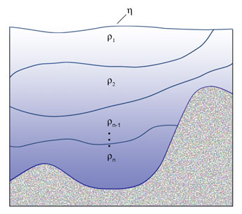
- isopycnal coordinates / layered models.
These models use the potential density referenced to
a given pressure as the vertical coordinate.
This system basically divides the water column into
distinct homogeneous layers, whose thicknesses can vary from place to place and from one time step to
the next.
This choice of coordinate works well for modeling tracer transport, which tends to
be along surfaces of constant density.
While both layered and isopycnal models use density as the vertical coordinate, there are subtle differences between the two types.
In a layered model, the outcropping of isopycnals is not permitted,
and layers are not permitted to vanish.
The chief advantage of layered models is their computational speed.
Because they are fast, they have been run at higher horizontal resolution,
and were the first type of model to
yield eddy-resolving simulations.
The chief disadvantage is that all the topography must be contained in the
lowest layer, so the ocean bottom can never be shallower than the depth
of the interface between the lowest two layers. This confines this class of models
to deep ocean basins and does not include continental shelf and slope regions.
In addition, since the density of each layer is invariant, this type of
model is not applicable to the surface mixed layer region where thermodynamic
processes such as heating/cooling and evaporation/precipitation change the
density.
In addition, they solve for density, rather than temperature and salinity
separately, so they assume a simple linear equation of state, and use the
same mixing and diffusion characteristics for temperature and salinity.
Isopycnal models are similar to layered models, but have overcome some of the numerical
problems that limit the layered models. They can have vanishing layers and
surfacing of the isopycnals, so that they can represent frontal regions more
accurately.
They also can have more complex bottom
topography, and a more realistic equation of state.
Water mass characteristics are preserved through
centuries of integration so this type of model is appropriate for use in large-scale global ocean climate models.
However, because
cross-isopycnal mixing is not allowed
in this type of model, this type of model has limited applicability in coastal
regions and in the surface and bottom boundary layers.
The z and sigma coordinates are Eulerian, i.e., they are fixed in space.
As such, they are more appropriate choices for
coastal models since they can more accurately resolve the top and bottom
boundary layers.
The layer and isopycnal coordinates are Lagrangian, i.e., they
change in position or thickness as a function of the dynamics.
They may be better suited to long-term simulations where preservation of
water mass characteristics are very important (Kantha and Clayson, 2000).
The three figures linked below from the
DYNAMO Report show how much the mixed layer depth can differ among
models with different vertical coordinates and different mixed layer parameterizations, even with identical domains,
spatial resolution and forcing.
Currently, there are three main vertical coordinates in use, none of which provides universal utility. Hence, many developers have been motivated to pursue research into hybrid approaches.
- Courtesy of Eric Chassignet (U. Miami)
Now that you have a grid defined in your model domain, the next step is to supply some "Boundary Conditions".