Now that you've made the necessary choices and built your model, it needs to be implemented on a computer somewhere. In this section, we'll look at the issues involved in the implementation of today's ocean models.
Because of the numbers of gridpoints in most ocean models, and the complexity of the equations that need to be solved, global ocean models are always pushing the limits of the largest and fastest computers of the day.
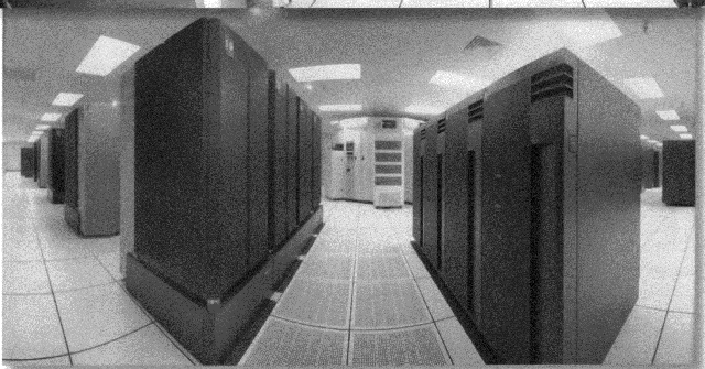
High Performance Computing is a term that refers to the capabilities of the biggest and fastest computers of the day. Today, this means thousands of processors with speeds of teraflops (1 teraflop is one trillion floating point operations per second), joined together and communicating with each other. In the mid-1990's, the Department of Defense established several Major Shared Resource Centers (MSRC's) across the country for DoD high performance computing applications. See http://www.hpcmo.hpc.mil. The MSRC at NAVO was established with a focus on ocean and weather prediction. The photograph below shows NAVO's IBM RS/6000 supercomputer - a two teraflop system with 1,336 processors and 1 gigabyte of memory per processor. It was the fourth largest supercomputer in the world in 2000.
Today's High Performance Computers are parallel computers. The term "parallel processing" refers to using multiple processors to solve a single problem, either by means of a supercomputer that contains many processors, or on a group of workstations that are networked together and share information. The advantages of parallel processing are
There are two types of parallel computer architecture:
|
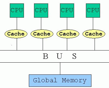
Shared Memory:
In a shared memory architecture, there is one huge bank of memory that is shared among all the processors (e.g. Origin 2000). |
|
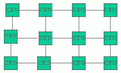
| Distributed Memory:
In a distributed memory architecture, each processor has its own memory, which is not shared with the other processors (e.g. IBM SP3). |
(After Foster, 1995) |
There are two main ways to parallelize your model code. The first is task parallelism, which means breaking the problem into a number of independent tasks and then each processor or group of processors can perform a separate task. The second method is data parallelism, in which the data or grid is divided into sections, so for example, each processor might compute the equations of motion on one line of longitude.
While the time required to run a model decreases as the number of processors increases, there is some overhead and efficiency lost because the processors have to pass information to each other. How efficiently this occurs as the number of processors change is known as scalability. If the number of processors doubles and the cpu time required is cut in half, then this is called perfect scalability. The graph below shows how the time required to obtain results in one global ocean model changes according to number of processors and the number of gridpoints.

In the figure above, courtesy McClean et al., 2001, the horizontal scale for the number of processors is logarithmic and ranges from 100 to 1000. The vertical axis is cpu seconds per time step, so naturally the fine resolution models (e.g. 0.1o) take longer. Perfect scalability is depicted by the green line. In the case of the coarser models, such as the barotropic 0.4o model case, the number of cpu seconds increases as processors are added. However, the fine resolution models gain the most from added processors because they have so many gridpoints.
Another issue to consider in implementation of a model is portability. Portability is the capability of the code to be moved from one computer architecture to another. Ideally, the code should be as portable as possible so that when a computer is upgraded or new computer is installed in a Center, few changes need to be made to the code. However, some models are designed to run more efficiently on one architecture and significant changes may need to be made if the code is ported to a different type of architecture.
In addition to high performance computing, there is a trend towards more distributed and local computing. For example, the PCTides model, discussed later in this course, is designed for local tide prediction and can run quickly on a desktop pc. A model such as this gives the user much more control as to the domain, resolution and forcing than submitting a request for a specific run to a Center. The future will most likely consist of a mixed computing environment, with some regional and local models being run on site, but with the global modeling and data assimilation being done centrally.
Congratulations! You really are done now - go ahead and click the "Done!" button.