
As you learned in the first section of this course, the real ocean moves in response to forces. These forces include the winds, tides, heating and cooling of the ocean surface, and precipitation and evaporation. In this section, we discuss how these forces are applied to the ocean in numerical models.
Wind "stress" is the quantity that is modifying the model's velocity field.
Units are dynes/cm2 [ = g/(cm s2) ] or
Newtons / m2 [ = kg/(m s2) ]
1 Pascal = 1 N/m2
1 dyne/cm2 = 0.1 N/m2

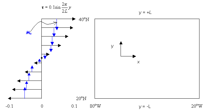
The schematic above depicts an idealized windstress for an ocean basin such as the North Atlantic. The blue arrows indicate the direction and relative magnitude of the Ekman transport.
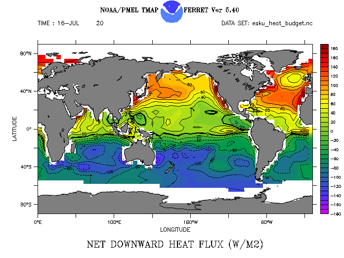
For comparison, see a global zonal windstress field from satellite scatterometer data.
Schematic of ocean movement from wind forcing
In simple terms - Newton's 2nd Law states:

If we express acceleration as the change in velocity with respect to time, we have:

or, rearranging terms:

Then

and we can solve for the new V at time2.
SO, what we use is wind STRESS - force of wind acting on a unit mass
There is no single formula to calculate windstress as a function of windspeed as a number of factors are involved, but in general, the windstress is proportional to the square of the windspeed. The constant of proportionality is called the drag coefficient. A 20 knot (~ 10 m/s) wind will produce a windstress on the order of 1 dyne/cm2.
Much of the the ocean's variability, especially in the top layers
are wind driven.
Realistic simulations REQUIRE realistic winds to be used.
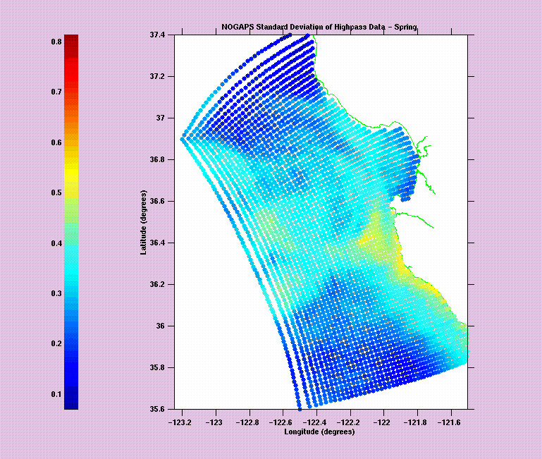
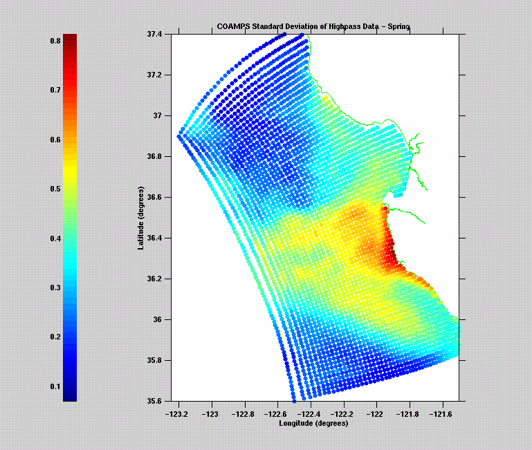
Ideally, the spatial resolution of the wind fields should match that of the ocean model. Practically speaking, global ocean models are usually forced with wind fields of 1 - 1.5o resolution. We are only now beginning to assess the impact of fine scale wind forcing on coastal ocean models. The two figures below illustrate how much more coastal SST variability there is (red colors) when the ocean is forced with 27 km resolution COAMPSTM winds versus 81 km NOGAPS winds. Note: on September 18, 2002, the resolution used in NOGAPS went from 0.75o to 0.50o, or from 81 km to 55 km resolution. According to FNMOC, "Testing confirmed the new model resolution provides a positive impact on the prediction of low level winds, precipitation, and tropical cyclone tracks in the tropics and some positive impact in the mid-latitudes."


These figures are courtesy of Jeff Paduan, (NPS).
We'll consider the various types of forcing on the ocean that can change the buoyancy of the water, first the heat flux and then the salt flux.
The temperature of the ocean varies spatially and temporally. Such changes indicate heat transfer by currents (advection), and heat loss and gain at the surface. The components of the surface heat flux are:
The three major sources of these flux values are:
A net heat flux, calculated from the four components produced by the atmospheric prediction models, is used to force the model. Fluxes can also be calculated from the observations using bulk formulae. Such fluxes have only become readily available recently. Earlier model efforts forced the sea surface temperature (SST) of the model back to observed climatological values. In a process known as restoring to climatology, ocean model surface temperatures were nudged back to monthly climatological values using a timescale of a month. High-frequency processes are absent using this type of forcing.
It is quite common to use observed or atmospheric prediction fluxes together with restoring, albeit with a longer restoring timescale, to avoid model "drift". This tends to be more of a concern for climate studies. In some cases, restoring can be turned on in an ocean-only model to mimic the effects of ice on the surface temperature in regions where ice would occur.
The whole issue of surface heat fluxes over the ocean is an important, and problematic, one for atmospheric, oceanic, and coupled models.
An example of the net heat flux from the ECMWF, and the four heat flux components:

The salinity of the surface waters are influenced by
Again, the first two fluxes are obtained from measurements and numerical weather prediction models. Examples from the same ECMWF Reanalysis climatology are:
Surface salinity is strongly influenced by the opposing effects of evaporation, which increases salinity, and precipitation, which decreases it. Finally, the influence of freshwater flow from rivers can be added into the salt balance. There is an annual river discharge database for the major rivers in the world (Perry et al., 1996). The river discharge goes into the model as point sources at the geographical locations of the river outflow.
Again, where river flow data or evaporation and precipitation information from NWP models is lacking, surface restoring of salinity to climatology is commonly used; alternatively, a combination of data, NWP fluxes, and restoring to climatology may be used to avoid model drift.
We have already talked some about tides in the ocean. Now we will talk about how tidal forcing is incorporated into numerical ocean models. In general global ocean circulation models do not include tides. There are special global ocean models designed just to predict the tidal sea surface elevation signal in the ocean. These use SSH data from satellite altimeters and coastal tide gauges and/or are forced by the tide generating force (or potential) that we discussed previously. The output from these global tidal models, which consists of tidal constants (amplitude and phase for many tidal constituents) throughout the domain is used to provide tidal forcing to regional ocean circulation and tide models.
The movie (from http://geodesy.eng.ohio-state.edu/tide.html) generated by Craig Tierney using the University of Texas CSR3.0 tide model represents the amplitudes of the M2, S2, K1, and O1 tide constituents. It covers four days with each frame separated by 1/2 hour. The beginning of the movie falls on 1 Jan 1992, 0 hr.
There are at least 4 ways in which tidal forcing is incorporated into regional ocean models.
Next, click on the "Initialization" button to see various ways a model may be started.