In order to solve a system of equations mathematically, boundary conditions need to be set. In addition to lateral, or side, boundary conditions, we will need to set
conditions at the ocean surface and bottom, but this will be addressed in
another section. There are three basic types of boundaries:
- Closed boundary - a natural candidate for a closed boundary would be a
coastline or possibly the shelf break. Physically, the condition is that no
water flows across the boundary. Closed boundary conditions can further be classified as
- no slip in which there is no flow along the boundary, as well as through it
or
- free slip in which there can be flow along the boundary, but not perpendicular, or
normal, to it.
- Open Boundary - In most models other than global models, we need
to set conditions for the sides of the domain not bounded by land.
While the conditions may be specified in a variety of ways, the goal
for open boundaries is to allow waves and disturbances originating within
the model domain to leave the domain without affecting the interior solution
in a way that is not physically realistic.
In some model configurations, we may also want "information", such as
sea level or velocity, to pass into the domain from the open boundary.
Here are some of the methods for
achieving open boundaries:
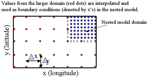
- Nested grids - in a nested grid, values at the grid points from the
larger model are used as boundary conditions at the appropriate locations
in the smaller nested model.
An atmospheric example that you might already be familiar with is a set of
a multiply-nested
COAMPSTM
grids which gets its outer boundary conditions from
NOGAPS
- Specified boundary conditions. Boundary conditions on open boundaries can be
specified or prescribed in a number of ways.
The boundaries can be set to climatological
values, which could be held constant or interpolated from say monthly values to
the time step of the model.
Observations obtained on a continuing basis can also be used.
This will be discussed further in the data assimilation section.
Prescribed forcing can also be applied on the open boundary.
PCTides,
for example,
varies sea level on the open boundary of the outermost domain according to tidal
constants derived from a global tidal model.
The Mediterranean Sea
SWAFS,
domain uses a
prescribed flow through the Straits of Gibraltar.
- Radiative or sponge boundaries - usually an additional set of gridpoints is used outside the actual
physical area of the model to help implement open boundary conditions.
In a sponge boundary, the idea is to absorb outward propagating waves and energy
rather than having it reflect back into the model domain.
- Periodic or Cyclic Boundary Conditions - This type of condition
is appropriate for channel flow. This condition is that
what goes out one side comes back in on the other.
This type of condition is often used to test models in development against
known analytic solutions.
Note: When using and interpreting model results, results near a boundary may
be questionable - if available, use a model where the area of interest
is in the interior of the model domain, well away from any boundary.
You're now ready to go on to the next section: Bathymetry.