The thermodynamic ice-ocean interaction parameterizations used by
McPhee
(2000) in 1-D Local Turbulence Closure (LTC) simulations of the Weddell Sea
Mixed Layer have been implemented in the LES to simulate the freezing and
melting of ice. A prescribed mean surface stress ![]() derived from
observations is applied at the upper model domain, and the velocity boundary
condition is nonslip in fluctuations with respect to the mean horizontal
velocity at the surface. Heat flux through the ice is also derived from ANZFLUX
measurements, and the model ocean heat flux at the upper boundary is
derived from
observations is applied at the upper model domain, and the velocity boundary
condition is nonslip in fluctuations with respect to the mean horizontal
velocity at the surface. Heat flux through the ice is also derived from ANZFLUX
measurements, and the model ocean heat flux at the upper boundary is
![]()
where the freezing point ![]() is the boundary temperature
is the boundary temperature ![]() is the LES
temperature in the first grid level adjacent to the boundary, and
is the LES
temperature in the first grid level adjacent to the boundary, and ![]() is a
nondimensional Stanton number, adjusted for consistency with vertical grid size
is a
nondimensional Stanton number, adjusted for consistency with vertical grid size
![]() .
Freezing and melting of ice is then determined by the imbalance between heat
fluxes in the ice and in the ocean.
.
Freezing and melting of ice is then determined by the imbalance between heat
fluxes in the ice and in the ocean.
Several LES runs have been carried out to test the stability of the upper ocean under conditions observed during ANZFLUX at certain times when ocean observations were not made. In general, they agree with the LTC results of McPhee (2000), showing the upper ocean becoming unstable to a process of thermobaric parcel detrainment, but at an earlier point in time. These simulations do not yet account for cabbeling effects, as this term was omitted in the preliminary simulations for comparison with LTC results.
Two of the first simulations are presented on a separate document.
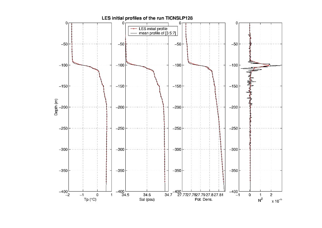
Simulation 3 was performed with a domain of 128x128x64 grid points, extended to
128x128x168 after one simulated day. The time step is 4s and the grid resolution 6m.
The LES was initialized from averaged typical profiles
measured in 1994 on year days 216 and 217 by the Turbulent Instrument Cluster and CTD,
and forced with time-dependent surface stress deduced from observations.
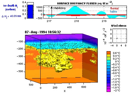
Potential temperature is shown on 2 vertical sections and two isothermal surfaces at 0°C
(above) and 0.4°C (below) representative of the pycnocline. The animation illustrates the evolution
of the plumes into a major convective cell that spreads when it reaches a level of neutral
buoyancy near 300m depth.
GIF Movie (5.0MB)
Figures 1-3 below summarize some results from this most recent simulation.
High wind in the first two days
results in shear production of mixed layer TKE with classical forced mixed
layer scaling, ![]() (Figure 1, top). Thermobarically unstable parcels are
subsequently detrained from the mixed layer in plumes with with small vertical
TKE, large negative skewness (Figure 1, second from top) and positive values of
(Figure 1, top). Thermobarically unstable parcels are
subsequently detrained from the mixed layer in plumes with with small vertical
TKE, large negative skewness (Figure 1, second from top) and positive values of
![]() below
below
![]() . Large
negative values of buoyant TKE production (Figure 1, third plot) resulting from
the conversion of TKE to entrainment work, are followed by significant release
of potential energy below the mixed layer as the detrained thermobaric plumes
become more negatively buoyant with depth. The fourth plot in Figure 1 tracks
the net buoyant production of TKE above and below
. Large
negative values of buoyant TKE production (Figure 1, third plot) resulting from
the conversion of TKE to entrainment work, are followed by significant release
of potential energy below the mixed layer as the detrained thermobaric plumes
become more negatively buoyant with depth. The fourth plot in Figure 1 tracks
the net buoyant production of TKE above and below ![]() separately, and
demonstrates that without thermobaricity the detrained plumes would be a net
sink, rather than a source of TKE. This sensitivity (lower right) to the second
order terms in the expanded equation of state arises from the high level of
compensation between the heat and salinity fluxes (lower left).
separately, and
demonstrates that without thermobaricity the detrained plumes would be a net
sink, rather than a source of TKE. This sensitivity (lower right) to the second
order terms in the expanded equation of state arises from the high level of
compensation between the heat and salinity fluxes (lower left).
Including the cabbeling term in the equation of state will probably
delay thermobaric instability, owing to the negative sign of ![]() for the plumes
(first results of this case can now be seen as an animation
here).
Mean TKE below the mixed layer is relatively small, but the skewness of the
thermobaric plumes is large and negative, and individual plumes (Figure 2) have
large downward velocities concentrated in structures about 100m in horizontal
scale.
for the plumes
(first results of this case can now be seen as an animation
here).
Mean TKE below the mixed layer is relatively small, but the skewness of the
thermobaric plumes is large and negative, and individual plumes (Figure 2) have
large downward velocities concentrated in structures about 100m in horizontal
scale.
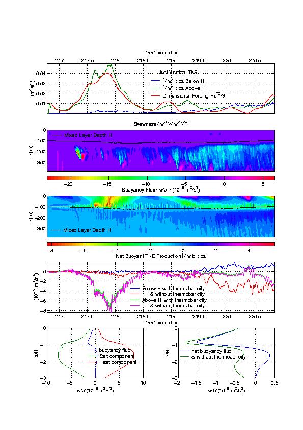
Figure 1: The top figure shows vertical TKE ![]() integrated over
depth, separately within and below the mixed layer, along with a representative
one-third of the dimensional surface stress forcing scale
integrated over
depth, separately within and below the mixed layer, along with a representative
one-third of the dimensional surface stress forcing scale ![]() . The profile
timeseries of mean skewness
. The profile
timeseries of mean skewness ![]() is illustrated in the second plot, and buoyancy
flux
is illustrated in the second plot, and buoyancy
flux ![]() -the work rate for buoyant TKE production- is shown in the
third plot. The fourth plot shows the net work rate due to buoyancy production
of TKE separately within and below the mixed layer, both with and without
thermobaricity. The lower right profile also shows the effect of thermobaricity
on buoyant TKE production, averaged over the entire simulation, and the lower
left plot decomposes
-the work rate for buoyant TKE production- is shown in the
third plot. The fourth plot shows the net work rate due to buoyancy production
of TKE separately within and below the mixed layer, both with and without
thermobaricity. The lower right profile also shows the effect of thermobaricity
on buoyant TKE production, averaged over the entire simulation, and the lower
left plot decomposes ![]() into heat and salinity flux components.
into heat and salinity flux components.

Figure 2: Vertical cross sections of potential temperature (top plot) and vertical velocity (bottom plot), on about day 220 of the simulation, illustrating a detraining thermobaric plume.