The LES model, developed by Deardorff (1980) and Moeng (1984) for the atmospheric boundary layer, dynamically solves for unresolved (subgrid) turbulent kinetic energy (TKE). Several adaptations of this model are currently used to model oceanic boundary layers, including high-latitude deep convection in response to storm forcing (Harcourt et al 2001), and forced convection in more shallow free-slip ocean boundary layers (e.g. Skyllingstad and Denbo, 1995; Wang et al, 1996).
Following Moeng (1984), the advection terms of the momentum equations
are computed prognostically from vorticity components ![]()
![]()
![]()
![]()
Terms involving both subgrid and resolved TKE are absorbed into a
modified nonhydrostatic pressure ![]() . b is the buoyancy force, and the mean
acceleration is removed from the right-hand side of the vertical momentum
equation to maintain a prescribed mean vertical velocity.
. b is the buoyancy force, and the mean
acceleration is removed from the right-hand side of the vertical momentum
equation to maintain a prescribed mean vertical velocity.
The LES uses a finite series expansion of the equation of state about a
potential reference state ![]() with density
with density ![]() chosen to
minimize truncation errors. After removing the horizontally averaged vertical
acceleration
chosen to
minimize truncation errors. After removing the horizontally averaged vertical
acceleration ![]() , buoyancy fluctuations
, buoyancy fluctuations ![]() account for
mean scalar dependence in the expansion coefficients, thermobaricity, cabbeling
and a ‘halobaric’ effect through
account for
mean scalar dependence in the expansion coefficients, thermobaricity, cabbeling
and a ‘halobaric’ effect through ![]() ,
, ![]() ,
, ![]() and
and ![]() , as
modifications to the standard approximation of constant thermal and haline
expansion coefficients
, as
modifications to the standard approximation of constant thermal and haline
expansion coefficients ![]() and
and ![]() . The salinity-related components of cabbeling and the
dependence of the haline expansion coefficient on mean salinity are small and
generally omitted.
. The salinity-related components of cabbeling and the
dependence of the haline expansion coefficient on mean salinity are small and
generally omitted.
The evolution of potential temperature is computed prognostically from
![]() with corresponding equations for salinity and Lagrangian tracers. The velocity
components are subject to the condition of incompressibility, which is applied
to the momentum equations to solve diagnostically for
with corresponding equations for salinity and Lagrangian tracers. The velocity
components are subject to the condition of incompressibility, which is applied
to the momentum equations to solve diagnostically for ![]() . Unresolved
stresses are modeled in terms of the symmetric resolved strain rate and local
nonlinear eddy viscosity
. Unresolved
stresses are modeled in terms of the symmetric resolved strain rate and local
nonlinear eddy viscosity ![]() ; scalar fluxes in terms of resolved gradients and eddy
diffusivity
; scalar fluxes in terms of resolved gradients and eddy
diffusivity ![]() :
:
Parameterizations eddy viscosity diffusivity, ![]() and
and ![]() , depend upon subgrid TKE
, depend upon subgrid TKE ![]() , its associated
dissipation length scale
, its associated
dissipation length scale ![]() , turbulent eddy Prandtl number
, turbulent eddy Prandtl number ![]() and constant
and constant
![]() . The
length scale
. The
length scale ![]() of unresolved motion is equal to the resolution scale
of unresolved motion is equal to the resolution scale ![]() , unless reduced
below that by stability or by proximity to a wall boundary. Parameterizations
for the dissipation length scale
, unless reduced
below that by stability or by proximity to a wall boundary. Parameterizations
for the dissipation length scale ![]() for stably stratified turbulence are discussed
below in the description of simulations. Resolution scale
for stably stratified turbulence are discussed
below in the description of simulations. Resolution scale ![]() is governed
either explicitly by a spatial filter, implicitly by the numerical scheme, or
by a combination of the two.
is governed
either explicitly by a spatial filter, implicitly by the numerical scheme, or
by a combination of the two.
The subgrid TKE equation
includes unresolved buoyant production ![]() as well as
unresolved shear production and transport, and parameterizes dissipation as
as well as
unresolved shear production and transport, and parameterizes dissipation as
![]() . When a
portion of the turbulent inertial subrange is resolved, constants
. When a
portion of the turbulent inertial subrange is resolved, constants ![]() and
and ![]() of the subgrid parameterization are determined by integrals
over the
of the subgrid parameterization are determined by integrals
over the ![]() Kolmogorov energy spectrum for unresolved TKE smaller than
Kolmogorov energy spectrum for unresolved TKE smaller than
![]()
The thermodynamic ice-ocean interaction parameterizations used by McPhee
(2000) in 1-D Local Turbulence Closure (LTC) simulations of the Weddell Sea
Mixed Layer have been implemented in the LES to simulate the freezing and
melting of ice. A prescribed mean surface stress ![]() derived from
observations is applied at the upper model domain, and the velocity boundary
condition is nonslip in fluctuations with respect to the mean horizontal
velocity at the surface. Heat flux through the ice is also derived from ANZFLUX
measurements, and the model ocean heat flux at the upper boundary is
derived from
observations is applied at the upper model domain, and the velocity boundary
condition is nonslip in fluctuations with respect to the mean horizontal
velocity at the surface. Heat flux through the ice is also derived from ANZFLUX
measurements, and the model ocean heat flux at the upper boundary is
![]()
where the freezing point ![]() is the boundary temperature
is the boundary temperature ![]() is the LES
temperature in the first grid level adjacent to the boundary, and
is the LES
temperature in the first grid level adjacent to the boundary, and ![]() is a
nondimensional Stanton number, adjusted for consistency with vertical grid size
is a
nondimensional Stanton number, adjusted for consistency with vertical grid size
![]() .
Freezing and melting of ice is then determined by the imbalance between heat
fluxes in the ice and in the ocean.
.
Freezing and melting of ice is then determined by the imbalance between heat
fluxes in the ice and in the ocean.
Several LES runs have been carried out to test the stability of the upper ocean under conditions observed during ANZFLUX at certain times when ocean observations were not made. In general, they agree with the LTC results of McPhee (2000), showing the upper ocean becoming unstable to a process of thermobaric parcel detrainment, but at an earlier point in time. These simulations do not yet account for cabbeling effects, as this term was omitted in the preliminary simulations for comparison with LTC results.
Figures 1-3 below summarize some results from the most recent
simulation, for which a short animation is available online at
http://www.oc.nps.edu/thermobaricity under Numerical Experiments,
Simulation 3. This simulation was initialized from averaged typical profiles
measured in 1994 on year days 216 and 217, and forced with time-dependent
surface stress deduced from observations. High wind in the first two days
results in shear production of mixed layer TKE with classical forced mixed
layer scaling, ![]() (Figure 1, top). Thermobarically unstable parcels are
subsequently detrained from the mixed layer in plumes with with small vertical
TKE, large negative skewness (Figure 1, second from top) and positive values of
(Figure 1, top). Thermobarically unstable parcels are
subsequently detrained from the mixed layer in plumes with with small vertical
TKE, large negative skewness (Figure 1, second from top) and positive values of
![]() below
below
![]() . Large
negative values of buoyant TKE production (Figure 1, third plot) resulting from
the conversion of TKE to entrainment work, are followed by significant release
of potential energy below the mixed layer as the detrained thermobaric plumes
become more negatively buoyant with depth. The fourth plot in Figure 1 tracks
the net buoyant production of TKE above and below
. Large
negative values of buoyant TKE production (Figure 1, third plot) resulting from
the conversion of TKE to entrainment work, are followed by significant release
of potential energy below the mixed layer as the detrained thermobaric plumes
become more negatively buoyant with depth. The fourth plot in Figure 1 tracks
the net buoyant production of TKE above and below ![]() separately, and
demonstrates that without thermobaricity the detrained plumes would be a net
sink, rather than a source of TKE. This sensitivity (lower right) to the second
order terms in the expanded equation of state arises from the high level of
compensation between the heat and salinity fluxes (lower left).
separately, and
demonstrates that without thermobaricity the detrained plumes would be a net
sink, rather than a source of TKE. This sensitivity (lower right) to the second
order terms in the expanded equation of state arises from the high level of
compensation between the heat and salinity fluxes (lower left).
Including the cabbeling term in the equation of state will probably
delay thermobaric instability, owing to the negative sign of ![]() for the plumes.
Mean TKE below the mixed layer is relatively small, but the skewness of the
thermobaric plumes is large and negative, and individual plumes (Figure 2) have
large downward velocities concentrated in structures about 100m in horizontal
scale.
for the plumes.
Mean TKE below the mixed layer is relatively small, but the skewness of the
thermobaric plumes is large and negative, and individual plumes (Figure 2) have
large downward velocities concentrated in structures about 100m in horizontal
scale.
We propose that this preliminary work on LES model development be extended through quantitative verification comparisons with existing data sets from polar boundary layers below ice, and subsequently be used to make predictions about upper ocean instabilities for use in designing future experiments in the Weddell Sea.
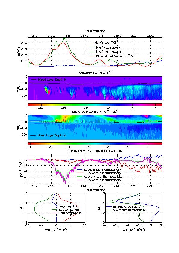
Figure 1: The top figure shows vertical TKE ![]() integrated over
depth, separately within and below the mixed layer, along with a representative
one-third of the dimensional surface stress forcing scale
integrated over
depth, separately within and below the mixed layer, along with a representative
one-third of the dimensional surface stress forcing scale ![]() . The profile
timeseries of mean skewness
. The profile
timeseries of mean skewness ![]() is illustrated in the second plot, and buoyancy
flux
is illustrated in the second plot, and buoyancy
flux ![]() -the work rate for buoyant TKE production- is shown in the
third plot. The fourth plot shows the net work rate due to buoyancy production
of TKE separately within and below the mixed layer, both with and without
thermobaricity. The lower right profile also shows the effect of thermobaricity
on buoyant TKE production, averaged over the entire simulation, and the lower
left plot decomposes
-the work rate for buoyant TKE production- is shown in the
third plot. The fourth plot shows the net work rate due to buoyancy production
of TKE separately within and below the mixed layer, both with and without
thermobaricity. The lower right profile also shows the effect of thermobaricity
on buoyant TKE production, averaged over the entire simulation, and the lower
left plot decomposes ![]() into heat and salinity flux components.
into heat and salinity flux components.

Figure 2: Vertical cross sections of potential temperature (left plot) and vertical velocity (right plot), on about day 220 of the simulation, illustrating a detraining thermobaric plume.
Preliminary LES model development has been guided by earlier development of the 1-D LTC model. While this has allowed some preliminary simulations, comparisons between the modified LES and observations of turbulence below the ice are necessary to verify the thermodynamic parameterizations of ice-ocean interaction. Data for verification will come from past observations of both ANZFLUX and SHEBA experiments. Comparisons will include vertical fluxes and dissipation rates as well as the evolution hydrographic profiles. Figure 3 demonstrates the equivalence of LES subgrid TKE dissipation and dissipation observations from a Turbulence Instrument Cluster (TIC) during the ANZFLUX experiment (n.b. two different time frames) by Tim Stanton and Miles McPhee.
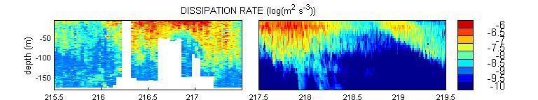
Figure 3: Time series of measured dissipation profiles (left plot) from the two final days of observation East of Maud Rise, along with LES subgrid dissipation (right plot) from the simulation of the subsequent two days, initialized from observed hydrographic profiles. Model resolution is 6.25m.
The two quantities are equivalent above the instrument noise level because the LES resolution scale is the same order as the length scale characterizing the TIC response, and because most of the dissipation is at much smaller length scales. We anticipate three verification simulations, two based on ANZFLUX observations and one based on SHEBA results, each about one week in duration. Ice-ocean parameterizations will be tuned to give the best agreement in these comparisons.
Modeling for predictions of upper ocean instabilities will focus on what may have happened in the area East of Maud Rise after the end of ANZFLUX ocean observations. This region is of interest because hydrographic analysis indicates a weak barrier to thermobaric instability if the upper ocean layer, and because satellite observations indicate significant areas of open water (Drinkwater, 1997) in 1994, and large polynyas in other years. The goal of this modeling is to use the dynamics of the LES predict more accurately the point at which instabilities occur and the form they will take. Furthermore, timeseries from ensembles of virtual measurements embedded in the LES will predict the shape of observed thermobaric plumes and other features of the upper ocean, and assess the random and systematic uncertainties associated with different observing systems. Embedded measurements will include Lagrangian, isobaric, and tethered Lagrangian drifter ensembles as well as Eulerian point and volume-averaged timeseries representing ice-fixed measurements.
In short, these embedded measurements will be used to assess the effectiveness of an array of experimental strategies, thus aiding in the design of future field expeditions. These virtual measurement ensembles will simulate observations in about six LES cases of one to two weeks in duration each, initialized from different 1994 ANZFLUX CTD profiles from East of Maud Rise, and forced with observed time-dependent surface forcing also derived from observations.
The LES code is currently optimized for parallelvector machines, where up to twothirds of the load is scalable. Each LES case, with 105 - 106 grid points model up to several weeks of simulation time (about 105 timesteps), and will require approximately 800 cpuhours on a Cray J90 or SV1, or 200 GAU in NCAR's general accounting units. In core memory requirements are moderate at 30MWords per simulation. These computer resources will be obtained through applications for the use of both NCAR and DOD high performance computing resources that are available to carry out NSF funded research. Large Eddy Simulations will be carried out by Harcourt and Lherminier, LTC simulations by McPhee. Analysis of model output for verification and prediction will be done by Harcourt, Lherminier, Stanton and McPhee.
Deardorff, J. W. (1980). Stratocumuluscapped mixed layers derived from a threedimensional model. Bound. Layer Meteor. 18, 495-527.
Drinkwater, M. R. (1997). Satellite microwave radar observations of climate-related sea-ice anomalies. Bull. Am. Met. Soc., Proc. Workshop on Polar Processes in Global Climate. 13-15 Nov. 1996, 115-118.
Harcourt, R. R., E. L. Steffen, R. W. Garwood, and E. A. D'Asaro (2001). Fully Lagrangian floats in Labrador Sea deep convection: Comparison of numerical and experimental results. J. Phys. Oceanogr. in press.
Moeng, C.H. (1984). A largeeddy simulation model for the study of planetary boundarylayer turbulence. J. Atmos. Sci. 41, 2052--2062.
Skyllingstad, E. and D. Denbo (1995). An ocean largeeddy simulation of Langmuir circulations and convection in the surface mixed layer. J. Geophys. Res. 100, 8501-8522.
Wang, D., W. G. Large, and J. C. McWilliams (1996). Largeeddy simulation of the equatorial ocean boundary layer: Diurnal cycling, eddy viscosity, and horizontal rotation. J. Geophys. Res. 101(C2), 3649-3662.