March 2002 deployment of the Autonomous Ocean Flux Buoy at the North Pole Enviromental Observation Station

The first ice deployment of an Autonomous Ocean Flux Buoy developed at NPS was made as a component of the North Pole Environmental Observatory during late April 2002. The following photographs and brief descriptions summarize the sequence of events leading to the deployment of the flux buoy at the very remote Arctic site near the North Pole.

[Outbound flight from Resolte Canada to Alert Canada, then ice station Borneo]

Getting there

Depolying instruments near the North Pole is complicated by the extreme remoteness of the site and the challenges of working in extreme low temperature conditions from a continually changing ice-covered ocean. Personnel and equipment were flown North from a staging area at Resolute Bay, NT, Canada, through Alert to Ice Camp Borneo on a chartered Hawker Siddley 748 run by First Air.

Ice Camp Borneo

The flux buoy was set in the ocean from a large, 2.5m thick multi-year ice pan about 1Km from Ice Camp Borneo. The Borneo ice camp is a runway and eco-tourist ice camp established at 89N, 90E in early March by Russian and French tour managers to support a range of Polar tourist activities. The camp provided runway and living support for 18 scientists and technicians executing the 2002 NPEO activities, which included recovering and redeploying an oceanographic mooring in 4Km of water, deploying 3 atmospheric and ice measurement stations, a Japanese upper ocean structure buoy, JCAD, and the NPS Ocean Flux Buoy.

Moving around the ice flow

Weight constraints prevented any snowmobiles and Nansen sleds from coming up to the ice camp, so instruments and deployment equipment was hauled out to the buoy site by Arkyo sleds. The buoy site was chosen after a survey to find the oldest and thickest multi-year ice which had the best chance of surviving ice cracking and ridging (and destruction of the buoys). The ice flow will crack, form leads and ridge as it moves out of the central Arctic toward the Atlantic Ocean over the next year. The cluster of meterological, ice flux and ocean buoys was assembled over a four day period.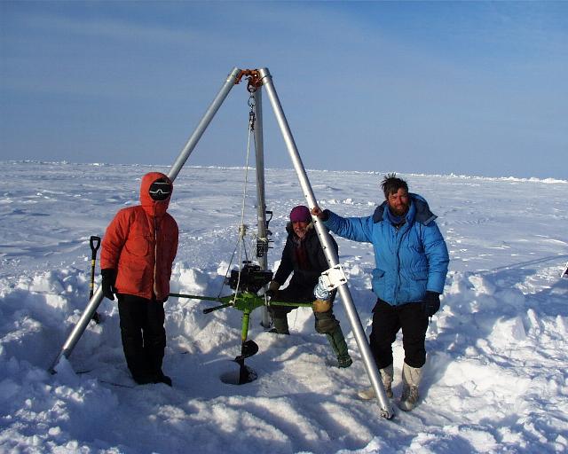

Drilling a 11" hole through the ice for the Flux buoy

A large power auger was used to drill a hole through the 8' thick ice. The tripod helped raise the auger when it cut through to the ocean before it could freeze in. The tripod and two hand winches were then used to lower the flux instrument sections into the ocean before being connected mechanically and electronically to the buoy housing.

Testing the Buoy

With the buoy physically deployed, each component of the buoy system was checked with a laptop computer in the wind break tent. By this time, winds were up to 30 knots with temperatures still - 30 C, so the tent provided important shelter to the buoy group out on the ice away from the camp. The full data stream from the flux buoy is periodically sent back to the Naval Postgraduate School by an Iridium satelite modem, which also provides two way communication to diagnose problems and change setups in the instrument system. If the Iridium link fails, a shorter data message is sent back by the older Argos satellite system. A Global Positioning System located with these antennas provides accurate time and position measurements every 15 minutes. The antennas for these systems are seen at the top of the buoy.

The deployed flux buoy

The buoy assembly was completed with a radome cover over the antennas to reduce snow buildup and provide some protection from potentially destructive Arctic foxes which have an unusual interest in our instrument systems. Measurments of ocean fluxes are made from an instrument cluster 4.5m below the ice within the 30-50m deep ocean mixed layer which sits above the strongly stratified halocline. A very low power acoustic travel time current sensor, a stable conductivity cell and a very high resolution thermistor measure velocities, salinity and temperature in the same small volume. Correlating fluctuations of vertical velocity with horizontal velocity fluctuations, temperature fluctuations and salinity fluctuations provide estimates of the vertical transport of momentum, heat and salt through the ocean mixed layer (see for example, McPhee and Stanton, Turbulence in the statically unstable oceanic boundary layer under Arctic leads, Journal of geophysical Research, pp6409-6428, March 1996).